Sharing articles

1. What the Federal Reserve Is and How It Works

Understanding the Federal Reserve System is the foundation for understanding interest rates, inflation, borrowing costs, stock market movements, and the overall U.S. economy. Before analyzing rate hikes, recessions, or market reactions, readers must clearly understand what the Federal Reserve is, how it is structured, and how it makes decisions.

This section builds that foundation in simple language, supported by real data and institutional facts.

1.1 What Is the Federal Reserve?

The Federal Reserve — often called “the Fed” — is the central bank of the United States. It manages the nation’s monetary system and influences how expensive or affordable borrowing money becomes across the entire economy.

The Fed was created in 1913 after a series of financial crises, especially the Panic of 1907, exposed weaknesses in the U.S. banking system. Congress passed the Federal Reserve Act to create a more stable financial structure.

At its core, the Fed has three primary responsibilities:

1. Set short-term interest rates
2. Maintain stable prices (control inflation)
3. Promote maximum sustainable employment

It is important to clarify that the Federal Reserve is not the same as the U.S. Treasury.

The U.S. Department of the Treasury manages government spending, collects taxes, and issues government debt. The Federal Reserve manages monetary policy and regulates the banking system. One controls fiscal policy (government budgets), the other controls monetary policy (money and interest rates).

As of the most recent data:

• The Federal Funds Rate target range reflects current monetary tightening or easing.
• Inflation (measured by CPI and PCE) shows whether price stability is being maintained.
• The unemployment rate reflects labor market strength.

These three indicators together define the Fed’s operating environment.

1.2 The Structure of the Federal Reserve System

The Federal Reserve is not a single institution located in one building. It is a system composed of multiple parts designed to balance regional and national economic interests.

There are three core components:

Board of Governors (Washington, D.C.)
The Board consists of seven members appointed by the U.S. President and confirmed by the Senate. Each member serves a 14-year term, designed to reduce political pressure and ensure independence.

The Chair of the Federal Reserve plays a central leadership role and represents the institution publicly. The Chair oversees policy direction and leads press conferences following interest rate decisions.

12 Regional Federal Reserve Banks
The country is divided into 12 Federal Reserve districts, including major cities such as:

• New York
• Chicago
• Dallas
• San Francisco
• Atlanta
• Boston

Each regional bank gathers economic data from its district, supervises banks, and contributes regional insights into national policy discussions. The New York Fed has a particularly important role because it conducts open market operations that implement interest rate decisions.

Federal Open Market Committee (FOMC)
The Federal Open Market Committee is the body that sets interest rates. It includes:

• The 7 Board of Governors members
• The President of the New York Fed
• 4 rotating presidents from the remaining regional banks

The FOMC meets eight times per year to evaluate economic data and vote on rate changes.

Board of Governors

The Board of Governors is the central governing body of the Federal Reserve System and serves as the core decision-making authority behind U.S. monetary policy. Located in Washington, D.C., the Board provides national oversight of the entire Federal Reserve structure and plays a leading role in setting interest rates, supervising banks, and maintaining financial stability.

The Board consists of seven members, known as Governors. Each Governor is nominated by the President of the United States and confirmed by the U.S. Senate. Governors serve staggered 14-year terms, which are intentionally long to protect the Federal Reserve from short-term political pressure. This structure ensures continuity and independence in monetary policy decisions.

One of the seven Governors is appointed as Chair of the Federal Reserve for a renewable four-year term. The Chair is the most visible leader of the Federal Reserve and serves as the primary spokesperson during press conferences, congressional testimony, and financial crises. The Chair also leads meetings of the Federal Open Market Committee (FOMC), which sets interest rate policy.

Another Governor is designated as Vice Chair, also serving a renewable four-year term. The Vice Chair supports the Chair and often leads initiatives related to financial regulation and stability.

There is also a Vice Chair for Supervision, a role created after the 2008 financial crisis to strengthen oversight of large financial institutions. This position focuses specifically on bank regulation, stress testing, capital requirements, and systemic risk monitoring.

Key Responsibilities of the Board of Governors:

Monetary Policy Leadership
All seven Governors are permanent voting members of the FOMC. This means they vote on every interest rate decision and policy action. Their collective votes heavily influence the direction of the Federal Funds Rate and overall monetary policy.

Banking Supervision and Regulation
The Board oversees large bank holding companies, supervises financial institutions, and sets regulatory standards. It establishes capital requirements, liquidity rules, and stress testing frameworks to ensure the stability of the U.S. banking system.

Financial Stability Oversight
The Board monitors risks within financial markets, including credit markets, asset bubbles, and systemic vulnerabilities. During crises, it can authorize emergency lending programs to stabilize markets.

Payment System Oversight
The Board supervises key national payment systems to ensure smooth financial transactions across the country.

Research and Data Analysis
The Board relies on extensive economic research, data modeling, and forecasting to guide decisions. Staff economists analyze inflation trends, labor markets, GDP growth, credit conditions, and global economic developments.

Independence and Structure

The staggered 14-year terms are one of the most important design features of the Board. Because only one term expires every two years, no single president can immediately reshape the entire Board. This reduces political influence and supports long-term economic stability.

Although Governors serve 14-year terms, the Chair and Vice Chair serve renewable four-year leadership terms within their broader tenure as Governors.

Governors cannot be removed for policy disagreements. They can only be removed for cause, which further strengthens institutional independence.

Geographic and Economic Representation

By law, the composition of the Board must reflect a broad representation of the U.S. economy, including agriculture, commerce, industry, services, and labor interests. This ensures decisions are not overly influenced by one region or sector.

Compensation and Funding

The Federal Reserve is self-funded. It does not receive appropriations from Congress. Instead, it earns income from interest on government securities and other assets. This funding structure further supports operational independence.

Why the Board of Governors Matters for Markets

Because all Governors vote at every FOMC meeting, their views on inflation, employment, and financial stability can strongly influence interest rate decisions. Markets closely watch speeches, testimony, and policy statements from Board members for signals about future rate hikes or cuts.

Investors analyze:

• Tone of public speeches
• Voting patterns
• Dissents during rate decisions
• Forecast changes in economic projections

A shift in Board leadership or vacancies can influence policy direction, making this body critically important for understanding future interest rate trends.

12 Regional Federal Reserve Banks

The 12 Regional Federal Reserve Banks are the operational arms of the Federal Reserve System. While the Board of Governors provides national leadership from Washington, D.C., the regional banks connect monetary policy to local economies across the United States.

When the Federal Reserve was created in 1913, lawmakers wanted to prevent financial power from being concentrated in one city. The result was a decentralized structure: twelve regional banks spread across different economic centers of the country. This ensures that monetary policy reflects conditions in manufacturing hubs, agricultural regions, energy-producing states, financial centers, and technology corridors.

The 12 Federal Reserve Districts and Their Head Offices:

1. Boston
2. New York
3. Philadelphia
4. Cleveland
5. Richmond
6. Atlanta
7. Chicago
8. St. Louis
9. Minneapolis
10. Kansas City
11. Dallas
12. San Francisco

Federal Reserve Districts and Their Key Economic Sectors

District	Federal Reserve Bank (Head City)	States / Major Coverage	Key Economic Sectors
1	Boston	New England (MA, CT, RI, VT, NH, ME)	Education, Healthcare, Biotechnology, Financial Services, Technology
2	New York	NY, Northern NJ, Puerto Rico, U.S. Virgin Islands	Global Finance, Investment Banking, Media, Real Estate, International Trade
3	Philadelphia	Eastern PA, Southern NJ, Delaware	Pharmaceuticals, Healthcare, Chemicals, Manufacturing, Financial Services
4	Cleveland	Ohio, Western PA, Eastern KY, Northern WV	Manufacturing, Automotive Parts, Steel, Healthcare
5	Richmond	VA, MD, NC, SC, DC, WV	Banking, Government Services, Agriculture, Manufacturing, Ports & Logistics
6	Atlanta	AL, FL, GA, Parts of TN, MS, LA	Tourism, Aerospace, Agriculture, Logistics, Consumer Services
7	Chicago	IL, IN, IA, WI, MI	Manufacturing, Agriculture, Automotive, Machinery, Financial Markets
8	St. Louis	MO, AR, Parts of IL, IN, KY, MS, TN	Agriculture, Food Processing, Transportation, Healthcare
9	Minneapolis	MN, MT, ND, SD, Parts of WI, MI	Agriculture, Energy, Mining, Banking, Manufacturing
10	Kansas City	CO, KS, NE, OK, WY, NM, Western MO	Energy (Oil & Gas), Agriculture, Aerospace, Transportation
11	Dallas	TX, Northern LA, Southern NM	Energy, Technology, International Trade (Mexico), Manufacturing
12	San Francisco	CA, OR, WA, AZ, NV, UT, ID, AK, HI	Technology, Venture Capital, Entertainment, Trade with Asia, Real Estate

The economic diversity across the 12 Federal Reserve districts ensures that U.S. monetary policy reflects the realities of technology-driven West Coast growth, Midwest manufacturing strength, Southern energy production, and Northeast financial markets. This decentralized structure allows regional economic data to influence national interest rate decisions.

Each regional bank serves a specific geographic district that includes multiple states. These districts reflect historical trade patterns rather than state boundaries.

Role and Core Responsibilities of Regional Federal Reserve Banks

Economic Research and Regional Intelligence
Each regional bank gathers economic data from businesses, community leaders, banks, and labor markets within its district. This “ground-level” information is shared with the Federal Open Market Committee (FOMC) before interest rate decisions.

For example:

• Manufacturing output in Chicago
• Agricultural activity in Kansas City
• Technology sector trends in San Francisco
• Energy production in Dallas

Current Presidents of the 12 Regional Federal Reserve Banks

District	Federal Reserve Bank	Current President
1	Federal Reserve Bank of Boston	Susan M. Collins
2	Federal Reserve Bank of New York	John C. Williams
3	Federal Reserve Bank of Philadelphia	Patrick T. Harker
4	Federal Reserve Bank of Cleveland	Loretta J. Mester
5	Federal Reserve Bank of Richmond	Thomas I. Barkin
6	Federal Reserve Bank of Atlanta	Raphael W. Bostic
7	Federal Reserve Bank of Chicago	Austan D. Goolsbee
8	Federal Reserve Bank of St. Louis	Alberto G. Musalem
9	Federal Reserve Bank of Minneapolis	Neel Kashkari
10	Federal Reserve Bank of Kansas City	Jeffrey R. Schmid
11	Federal Reserve Bank of Dallas	Lorie K. Logan
12	Federal Reserve Bank of San Francisco	Mary C. Daly

The President of the New York Fed (John C. Williams) serves as a permanent voting member of the Federal Open Market Committee (FOMC), while the remaining regional presidents rotate voting responsibilities annually.

This real-time feedback ensures policy decisions are not based solely on national averages but also reflect regional economic conditions.

Bank Supervision and Regulation
Regional Fed banks supervise and regulate member banks within their districts. They examine financial institutions to ensure they meet capital, liquidity, and risk management standards.

They also conduct stress testing, coordination, and monitor financial stability risks within their jurisdictions.

Financial Services to Banks and the Government
Regional banks provide essential services such as:

• Processing checks and electronic payments
• Distributing and collecting U.S. currency
• Managing government accounts
• Operating components of the national payments infrastructure

They act as the “bank for banks,” helping ensure liquidity flows smoothly through the financial system.

Implementation of Monetary Policy
While the FOMC sets policy, regional banks help implement it.

The most important operational role belongs to the Federal Reserve Bank of New York. Through its trading desk, it conducts open market operations — buying and selling U.S. Treasury securities to maintain the target federal funds rate.

Because of this responsibility, the President of the New York Fed is a permanent voting member of the FOMC.

Leadership Structure of Regional Banks

Each regional bank has:

• A President
• A Board of Directors

The President of each regional bank participates in FOMC meetings. However, only five regional presidents vote at any given time:

• The New York Fed President (permanent voter)
• Four other regional presidents (rotate annually)

This rotation system ensures geographic balance in monetary policy decisions.

Funding Structure

Regional Federal Reserve Banks are not funded by taxpayer dollars. Like the broader Federal Reserve System, they generate income primarily from interest on government securities and other financial assets.

After covering operating expenses, surplus earnings are transferred to the U.S. Treasury.

Why Regional Banks Matter for Interest Rates and Markets

Financial markets pay close attention to speeches and economic commentary from regional Fed presidents. Their public statements often signal future policy direction.

For example:

• A “hawkish” regional president may signal support for rate hikes to fight inflation.
• A “dovish” president may signal support for rate cuts to stimulate growth.

These signals can move:

• Stock markets
• Bond yields
• Currency markets
• Commodity prices

The Beige Book

One important contribution of regional banks is the Beige Book — a report published eight times per year summarizing economic conditions in each district. This report provides qualitative insights on:

• Consumer spending
• Wage pressures
• Hiring conditions
• Supply chain issues
• Credit demand

The Beige Book is widely followed by economists, investors, and policymakers because it reflects real-time economic sentiment.

Economic Diversity Across Districts

Each district represents a different economic strength:

• New York: Finance and global banking
• Chicago: Manufacturing and agriculture
• Dallas: Energy production
• San Francisco: Technology and innovation
• Atlanta: Transportation and logistics

This diversity ensures monetary policy decisions reflect the complexity of the U.S. economy.

Federal Open Market Committee (FOMC)

The Federal Open Market Committee (FOMC) is the body within the Federal Reserve System that makes official decisions about U.S. monetary policy — including whether interest rates go up, go down, or stay the same. When people hear that “the Fed raised rates” or “the Fed cut rates,” that decision was made by the FOMC.

The FOMC is the most powerful monetary policy committee in the world because its decisions directly influence borrowing costs, inflation, employment levels, stock markets, bond yields, currency strength, and global capital flows.

What the FOMC Actually Does

The FOMC’s primary responsibility is to set the target range for the Federal Funds Rate — the benchmark short-term interest rate that influences nearly every other rate in the U.S. economy.

However, its responsibilities go beyond just rate decisions. The FOMC:

• Sets the Federal Funds Rate target range
• Oversees open market operations (buying and selling U.S. Treasury securities)
• Directs quantitative easing (QE) or quantitative tightening (QT) programs
• Evaluates inflation, employment, and financial stability
• Provides forward guidance to financial markets
• Publishes economic projections and policy outlooks

In short, the FOMC controls the direction of U.S. monetary conditions.

Composition of the FOMC

The FOMC consists of 12 voting members:

• The 7 members of the Board of Governors
• The President of the Federal Reserve Bank of New York (permanent voter)
• 4 of the remaining 11 Regional Federal Reserve Bank presidents (rotating annually)

Although only 12 members vote, all 19 participants (7 Governors + 12 Regional Presidents) attend meetings and contribute to discussions.

This structure balances national oversight with regional economic input.

How the FOMC Makes Decisions

The FOMC meets eight times per year on a scheduled calendar. Emergency meetings can also occur during financial crises.

Before each meeting:

1. Regional banks gather economic data from businesses, banks, labor markets, and industries in their districts.
2. Staff economists prepare detailed reports analyzing inflation, GDP, employment, financial markets, and global conditions.
3. The Beige Book is distributed, summarizing regional economic conditions.

During the meeting:

• Members review data.
• Economic forecasts are presented.
• Risks are debated (inflation risk vs recession risk).
• Members vote on policy actions.

Decisions are made by majority vote.

If there is disagreement, dissenting votes are recorded publicly. Financial markets pay close attention to dissents because they signal internal policy divisions.

Key Tools Directed by the FOMC

Federal Funds Rate Target
The FOMC sets a target range (for example, 5.25%–5.50%). The New York Fed then conducts operations to keep the actual rate within that range.

Open Market Operations
The FOMC authorizes the buying and selling of U.S. Treasury securities to manage liquidity in the banking system.

Quantitative Easing (QE)
During economic downturns, the FOMC may authorize large-scale asset purchases to inject liquidity into financial markets.

Quantitative Tightening (QT)
To reduce inflation or normalize policy, the FOMC may allow its balance sheet to shrink by not reinvesting maturing securities.

Forward Guidance
The FOMC provides signals about future policy direction through official statements and press conferences. Phrases such as “data dependent” or “higher for longer” can move markets significantly.

Economic Projections and Transparency

Four times per year, the FOMC releases the Summary of Economic Projections (SEP). This includes:

• Inflation forecasts
• GDP growth projections
• Unemployment expectations
• Federal Funds Rate projections (Dot Plot)

The “Dot Plot” shows each voting member’s expectations for future interest rates. Markets analyze the median projection to anticipate future rate moves.

After each meeting, the FOMC releases:

• A policy statement
• A vote breakdown
• An explanation of economic conditions
• A press conference by the Fed Chair

Meeting minutes are published three weeks later, providing deeper insight into policy debates.

Why the FOMC Matters for Financial Markets

Every FOMC decision can impact:

Stock Market
Higher rates often pressure growth stocks due to higher discount rates. Lower rates tend to support equities.

Bond Market
Bond prices move inversely to interest rate expectations. A rate hike typically pushes yields higher and bond prices lower.

Mortgage Rates
Changes in rate expectations influence 10-year Treasury yields, which affect mortgage rates.

U.S. Dollar
Higher rates often strengthen the dollar because global investors seek higher returns.

Commodities and Gold
Gold prices often move inversely with real interest rates.

Historical Importance of the FOMC

Over the decades, the FOMC has:

• Raised rates aggressively to fight 1980s inflation
• Cut rates to near zero during the 2008 financial crisis
• Launched quantitative easing programs
• Cut rates to zero during the 2020 pandemic
• Rapidly rising rates during the 2022–2024 inflation surge

These actions reshaped global markets and economic cycles.

Voting Rotation System

The President of the New York Fed votes permanently because that bank implements open market operations.

The other regional presidents rotate voting annually in groups, ensuring geographic diversity.

Even when not voting, non-voting presidents still participate in discussions and influence policy direction.

How Investors Monitor the FOMC

Professional investors track:

• Changes in policy statement language
• Economic forecast revisions
• Dot Plot shifts
• Dissents
• Tone during press conferences
• Balance sheet policy adjustments

Even a small wording change in the FOMC statement can trigger major stock and bond market reactions.

Current FOMC Voting Members (2026 Update)

Each year, the Federal Open Market Committee updates which regional Federal Reserve Bank presidents will have voting rights in addition to the Board of Governors and the permanent New York Fed vote. Voting membership for 2026 was determined at the first regularly scheduled FOMC meeting of the year.

For 2026, the FOMC voting members include:

The Federal Open Market Committee (FOMC) consists of 12 voting members. These members are responsible for setting the Federal Funds Rate and directing U.S. monetary policy. The voting structure combines national leadership with regional representation.

Chair: Jerome H. Powell
Vice Chair: Philip N. Jefferson
Vice Chair for Supervision: Michael S. Barr

Board Governors:
• Michelle W. Bowman
• Lisa D. Cook
• Adriana D. Kugler
• Christopher J. Waller

President of the Federal Reserve Bank of New York (Permanent Voting Member):
• John C. Williams

Rotating Regional Federal Reserve Bank Presidents Voting in 2026:

• Federal Reserve Bank of Cleveland – Loretta J. Mester
• Federal Reserve Bank of Dallas – Lorie K. Logan
• Federal Reserve Bank of Minneapolis – Neel Kashkari
• Federal Reserve Bank of Philadelphia – Patrick T. Harker

All other Regional Federal Reserve Bank presidents attend FOMC meetings and participate in policy discussions, but do not vote in 2026. The voting rotation changes annually at the first scheduled FOMC meeting of the year.

Key Information for Readers

• Current FOMC voting members and leadership roles
• Upcoming FOMC meeting calendar (eight scheduled meetings per year)
• Annual regional voting rotation schedule

Permanent FOMC Voters
These members vote every year because of their roles:

• All seven Board of Governors members
• President of the Federal Reserve Bank of New York (permanent regional voter)

Rotating Regional Fed Presidents (2026)
Four additional regional bank presidents rotate in each year. For 2026, the voting regional presidents are:

• President, Federal Reserve Bank of Cleveland
• President, Federal Reserve Bank of Dallas
• President, Federal Reserve Bank of Minneapolis
• President, Federal Reserve Bank of Philadelphia

Non-voting Participants
All other Regional Fed presidents participate in policy discussions and economic analysis at FOMC meetings, but do not cast a vote in 2026.

How the Rotation Works

• The president of the Federal Reserve Bank of New York is always a voting member.
• Of the remaining 11 regional Fed presidents, four receive voting rights each year, rotating on a scheduled cycle to ensure geographic representation.
• This rotation changes annually at the first regularly scheduled FOMC meeting (usually January).

2026 Rotating In (Voting This Year)

• Cleveland Fed President
• Dallas Fed President
• Minneapolis Fed President
• Philadelphia Fed President

2026 Rotating Out (Non-voting This Year)
Presidents not voting in 2026 include those from:

Kansas City

Boston

Chicago

St. Louis

1.3 The Fed’s Dual Mandate

The foundation of U.S. monetary policy rests on what is called the “dual mandate.” This mandate was given to the Federal Reserve System by Congress and defines the two core objectives that guide every interest rate decision, policy adjustment, and economic forecast.

In simple terms, the Federal Reserve has two main goals:

1. Maximum Employment
2. Stable Prices

Every FOMC meeting, every rate hike or rate cut, and every economic projection is evaluated through the lens of these two objectives.

Maximum Employment: What It Really Means

Maximum employment does not mean zero unemployment. In a dynamic economy, some level of unemployment is normal and even healthy. People change jobs, relocate, graduate from school, or temporarily leave the workforce. Economists refer to this as “frictional unemployment.”

The Fed aims for what is often called the “natural rate of unemployment” — the lowest level of unemployment the economy can sustain without causing excessive inflation.

If unemployment is too high:

• Consumer spending slows
• Business revenues fall
• Economic growth weakens

If unemployment is too low:

• Labor shortages emerge
• Wages rise rapidly
• Inflation pressures increase

The Fed’s challenge is to keep the labor market strong without allowing it to overheat.

Key Labor Market Indicators You Should Include

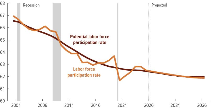
Unemployment Rate
This measures the percentage of people actively seeking work but unable to find jobs. It is one of the most closely watched economic indicators.

Nonfarm Payroll Growth
Released monthly, this measures how many jobs were added or lost in the economy, excluding farm workers.

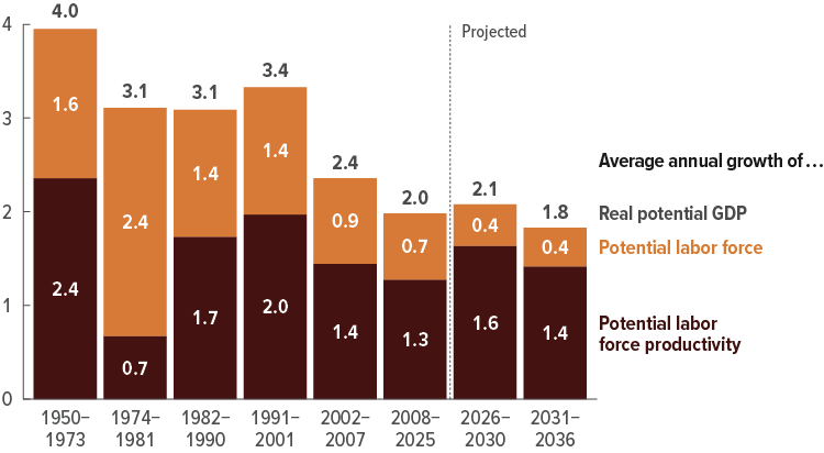
Labor Force Participation Rate
This shows the percentage of working-age individuals either employed or actively looking for work. A declining participation rate can signal structural labor issues.

Job Openings (JOLTS Data)
The Job Openings and Labor Turnover Survey shows how many positions employers are trying to fill. High job openings often indicate strong labor demand.

Average Hourly Earnings
Wage growth is critical. Rapid wage increases can boost consumer spending but may also create inflationary pressure.

By analyzing these data points together, the Fed determines whether the labor market is balanced, overheating, or weakening.

Stable Prices: Controlling Inflation Without Stopping Growth

The second part of the dual mandate is price stability — keeping inflation under control.

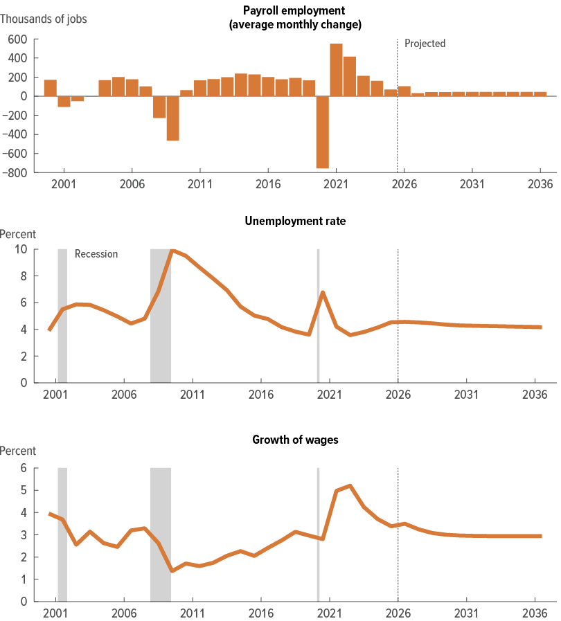
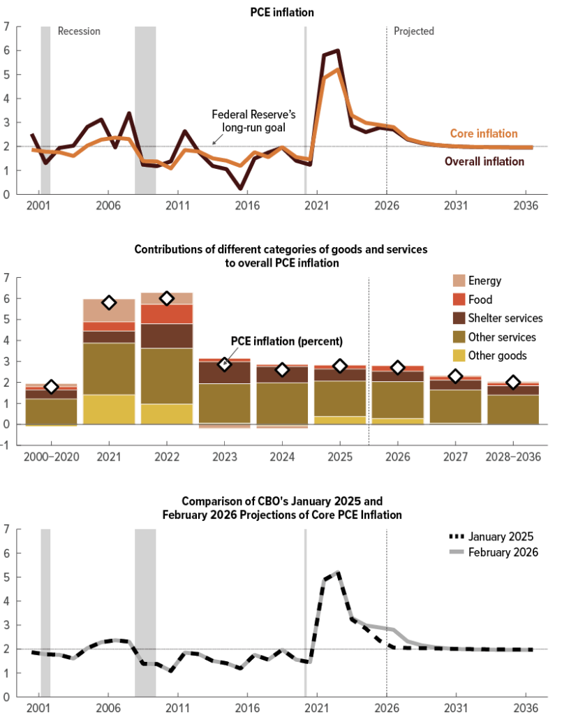
The Federal Reserve has defined its long-term inflation target as 2 percent. This target is measured primarily using the Personal Consumption Expenditures (PCE) price index.

Why 2 percent and not 0 percent?

Zero inflation may sound ideal, but mild inflation supports economic growth. A small, predictable level of inflation:

• Encourages consumer spending
• Supports wage growth
• Prevents deflation (a sustained decline in prices)

Deflation can be dangerous because it encourages people to delay purchases, which slows economic activity and investment.

If inflation rises well above 2 percent:

• Purchasing power declines
• Consumer confidence falls
• Interest rates often rise

If inflation falls too low:

• Economic growth can stall
• Businesses reduce investment
• Wages stagnate

Important Inflation Indicators You Should Include

Consumer Price Index (CPI)
Measures price changes for a basket of goods and services. Often used in media reports.

Core CPI
Excludes food and energy prices, which can be volatile.

PCE Inflation
The Fed’s preferred inflation measure. It adjusts for changes in consumer behavior and provides a broader view of spending patterns.

Core PCE
Excludes food and energy, offering a clearer view of underlying inflation trends.

Markets pay close attention to whether inflation readings are above or below the 2 percent target, as this heavily influences interest rate decisions.

How the Dual Mandate Shapes Interest Rate Decisions

When inflation rises above target and unemployment is low, the Fed may raise interest rates to cool demand and prevent overheating.

When unemployment rises, and inflation is stable or falling, the Fed may lower interest rates to stimulate economic growth.

This balancing act is often described as achieving a “soft landing” — slowing inflation without causing a recession.

However, policy trade-offs exist. Tightening policy too aggressively can push the economy into recession. Acting too slowly can allow inflation to become entrenched.

Dual Mandate Snapshot (Latest U.S. Data)

Inflation (PCE)

• Current Level: 2.8%
• Fed Target: 2.0%
• 10-Year Average: ~2.2%
• Status: Above Target

Core PCE Inflation

• Current Level: 2.8%
• Fed Target: 2.0%
• 10-Year Average: ~2.2%
• Status: Above Target

Unemployment Rate

• Current Level: 4.3%
• Fed Estimated Natural Rate: ~4.0%–4.5%
• 10-Year Average: ~5.0%
• Status: Near Balanced

Wage Growth (Average Hourly Earnings)

Status: Moderate Growth

Current Level: ~$31.95/hour

Stable Growth Range: Aligned with ~2% inflation

10-Year Average: ~$31/hour

This table immediately shows readers whether the economy is running “hot,” “cool,” or near equilibrium.

Why the Dual Mandate Matters for Small Businesses, Consumers, and Investors

For Small Businesses
Higher interest rates increase borrowing costs and can slow demand. Lower rates reduce financing costs but may increase wage pressures.

For Consumers
Interest rate changes affect mortgages, credit cards, car loans, and savings returns.

For Investors
Stock valuations, bond yields, and currency markets respond directly to expectations about inflation and employment trends.

Final Perspective

The dual mandate is the compass guiding all Federal Reserve policy decisions. Understanding maximum employment and stable prices gives readers the framework to interpret future rate hikes, cuts, and economic projections.

Every policy decision ultimately answers one question:

Is the economy too hot, too cold, or balanced?

The Federal Reserve’s job is to adjust monetary conditions until those two goals — strong employment and stable prices — move back into alignment.

1.4 How Monetary Policy Actually Works

Monetary policy may sound complex, but at its core, it relies on a few key tools that the Federal Reserve System uses to influence borrowing costs, liquidity, and economic activity in the United States. Each tool affects the economy through different channels — from the cost of loans to banks’ willingness to lend, to the amount of money circulating in financial markets.

Federal Funds Rate

The Federal Funds Rate is the central interest rate that banks charge each other for overnight loans of reserve balances. It is the most visible monetary policy tool because it sets the baseline cost for short-term borrowing in the economy. The Federal Open Market Committee (FOMC) sets a target range for this rate at every scheduled meeting.

As of the January 2026 FOMC meeting, the target range for the federal funds rate is 3.50% to 3.75% — unchanged from the previous meeting after a series of rate changes in the last few years aimed at balancing inflation and growth.

When the Fed raises the Federal Funds Rate:

• Mortgage rates tend to rise
• Credit card interest rates go up
• Business borrowing costs increase
• Overall borrowing slows

This typically cools consumer spending and business investment.

When the Fed lowers the Federal Funds Rate:

• Borrowing becomes cheaper
• Businesses may expand
• Consumers are more likely to finance purchases
• Economic activity is stimulated

This is why central banks often cut rates during slowdowns and raise them when inflation pressures rise.

Open Market Operations

Open Market Operations (OMOs) are the Fed’s most frequently used tool for implementing its monetary policy target. The Federal Reserve buys or sells U.S. Treasury securities in financial markets to influence the supply of money and the level of interest rates.

• Buying securities injects money into the banking system, increasing liquidity and generally lowering interest rates.
• Selling securities removes money from the system, tightening liquidity and placing upward pressure on interest rates.

The New York Fed conducts these operations on behalf of the FOMC to ensure the effective federal funds rate stays within its target range.

Discount Rate

The discount rate is the interest rate charged by the Federal Reserve when commercial banks borrow directly from the Fed’s discount window. This tool is primarily used as a safety valve for bank liquidity. The discount rate is typically set above the federal funds rate to encourage banks to seek funding from other banks first and to use the discount window only when necessary.

Reserve Requirements

Banks are historically required to hold a certain percentage of their deposits on reserve — either as cash in vaults or as deposits with the Federal Reserve. These reserve requirements affect how much money banks can lend. While this tool is rarely changed in day-to-day policy today, it remains part of the Fed’s toolkit for adjusting overall credit in the system.

Quantitative Easing (QE) and Quantitative Tightening (QT)

When interest rates were already near zero in past crises, the Federal Reserve turned to Quantitative Easing (QE) — large-scale purchases of Treasury securities and mortgage-backed securities — to inject liquidity and support financial markets and borrowing conditions. Over time, these QE programs expanded the Fed’s balance sheet dramatically. For example, the balance sheet grew from under $1 trillion before 2008 to around $4 trillion after QE programs in the early 2010s.

During the COVID-19 pandemic, the Fed again expanded its balance sheet significantly, leading to a peak total assets figure nearing $9 trillion in 2022 before policy normalization began.

In contrast, Quantitative Tightening (QT) is the process by which the Fed reduces its balance sheet by allowing securities to mature without reinvesting the proceeds. Starting from its historic peaks following the pandemic, the Fed has allowed much of this portfolio to shrink, bringing total assets down to around $6.6 trillion by late 2025 as part of policy normalisation.

These large asset purchases (QE) and runoff programs (QT) change the amount of reserves in the banking system and thereby affect market interest rates, credit conditions, and long-term borrowing costs beyond the federal funds rate alone.

Putting It All Together: A Flow Diagram

Here’s the basic transmission mechanism for monetary policy:

Fed decision → Change in cost of bank funding → Change in interest rates for businesses & consumers → Spending & investment reaction → Impact on inflation & employment

For example:

• When the Fed tightens policy (“hawkish”), credit becomes more expensive, slowing demand and putting downward pressure on inflation, but possibly slowing job growth.
• When the Fed loosens policy (“dovish”), borrowing becomes cheaper, stimulating spending and investment, potentially boosting jobs — but too much can push inflation above target.

This framework shows how the Fed’s policy tools — from the federal funds rate to QE/QT — operate through financial markets and the real economy to steer growth, inflation, and labor markets in line with its dual mandate.

1.5 Key Economic Indicators the Fed Watches

The Federal Reserve is fundamentally data-driven. Every interest rate decision, policy pivot, or forward-guidance statement depends on measurable economic indicators that signal the health of the U.S. economy. Policymakers do not guess — they evaluate hard data on inflation, jobs, growth, and financial stability before acting.

Below are the most important indicators the Fed watches closely, along with recent figures to give your readers context.

Inflation Indicators

Inflation measures changes in the prices consumers and businesses pay for goods and services. The Fed’s policy decisions are heavily influenced by whether inflation is above, near, or below the long-term target of 2 percent.

Consumer Price Index (CPI)

• CPI tracks a broad basket of goods and services out-of-pocket by consumers.
• Latest reading (Dec 2025): 3.4% year-over-year (U.S. Bureau of Labor Statistics) — above the Fed’s 2% target.

Core CPI (excludes food and energy)

• Often used to strip out volatile items.
• Latest reading (Dec 2025): 3.7% y/y — shows underlying inflation pressures.

Personal Consumption Expenditures (PCE) Price Index

• The Fed’s preferred inflation measure is the one that reflects consumer spending patterns in greater detail.
• Latest PCE inflation (Nov 2025): 2.8% y/y (Bureau of Economic Analysis).

Core PCE (excludes food and energy)

• This sub-measure is watched most closely at the Fed — it lines up closely with policy goals.
• Latest Core PCE (Nov 2025): 2.8% y/y.

Together, these inflation gauges show that price pressures remain above the Fed’s 2% goal, which informs decisions to slow the pace of rate cuts or maintain higher policy rates longer.

Employment Indicators

Strong employment is a central part of the Fed’s dual mandate. The Fed tracks multiple labor market metrics to separate healthy job growth from overheating or weakening conditions.

Nonfarm Payrolls

• Measures monthly job gains and losses across most sectors (excludes farm workers).
• Latest data (Jan 2026): +182,000 jobs added — moderate job growth.

Unemployment Rate

• Percentage of people actively seeking but unable to find work.
• Jan 2026: 4.3% (Bureau of Labor Statistics) — historically low, near full employment.

Wage Growth (Average Hourly Earnings)

• Wage growth signals labor market tightness.
• Latest: 4.1% y/y — moderate wage increases, but not at historic highs.

Labor Force Participation Rate

• The percentage of working-age people either working or looking for work.
• Latest: 62.6% — still below pre-COVID levels, suggesting some slack in the labor market.

These indicators help the Fed evaluate whether the labor market is too tight (which can fuel inflation) or too weak (which can drag on growth).

Growth Indicators

Growth metrics help the Fed determine whether the economy is expanding, slowing, or at risk of recession.

Gross Domestic Product (GDP)

• The broadest measure of economic activity.
• Latest real GDP growth estimate (Q4 2025): ~2.1% annualized — moderate growth.

Retail Sales

• Tracks consumer spending, which accounts for about two-thirds of GDP.
• Latest monthly retail sales growth: 0.3% — steady consumer demand.

Industrial Production

• Measures output in manufacturing, mining, and utilities.
• Latest: 0.1% increase month-over-month — stable industrial activity.

Together, these indicators help the Fed assess whether economic growth is broad-based or uneven.

Financial Stability Indicators

Monetary policy also considers risks within financial markets that could disrupt credit, lending, or liquidity.

Yield Curve (2-Year vs 10-Year Treasury Spread)

• The yield curve shows the relationship between short-term and long-term interest rates.
• When the 2-year rate exceeds the 10-year rate (an inversion), it has historically signaled recession risk.
• As of early 2026, the yield curve remains slightly inverted, which signals cautious market sentiment.

Credit Spreads

• The difference between corporate bond yields and Treasury yields.
• Widening spreads signal greater risk aversion in markets.

Bank Lending Standards

• Collected through the Fed’s Senior Loan Officer Opinion Survey (SLOOS).
• Tighter standards indicate banks are less willing to lend — a sign of financial contraction.

These indicators are not part of the dual mandate but are critical for detecting emerging stress in the financial system.

Why These Indicators Matter

When inflation remains above the Fed’s target, and the labor market is strong, policymakers may delay cutting rates or hold rates steady to prevent the economy from overheating.

If inflation eases while job growth slows, the Fed may be more comfortable reducing rates to support growth.

Financial stability measures (like the yield curve) add another layer — signaling when markets may be pricing in a recession, which can prompt pre-emptive policy action.

2. How Interest Rates Are Set and Why They Change

2.1 What Is the Federal Funds Rate?

The Federal Funds Rate is the most influential short-term interest rate in the U.S. financial system. It is the interest rate at which depository institutions (banks, credit unions, savings institutions) lend reserve balances to each other overnight. This rate influences borrowing costs across the economy — including mortgages, auto loans, credit card rates, and business lending — making it one of the Fed’s primary policy tools.

The Federal Funds Rate is the rate at which banks lend reserve balances (their cash held at Federal Reserve banks) to other banks with short-term funding needs. Because banks must maintain certain reserve levels, when they are short on reserves, they borrow from other institutions that have excess.

The Federal Open Market Committee (FOMC) does not set the actual rate directly. Instead, it establishes a target range for the rate and uses market operations to guide the effective rate toward that target.

Target Range Explanation

Instead of announcing a single fixed rate, the Fed announces a target range for the Federal Funds Rate. For example:

• At the January 2026 FOMC meeting, the target range was set at 3.50%–3.75%.
• This range reflects the Federal Reserve’s current stance on monetary policy — balancing inflation control and economic growth.

The Federal Reserve uses tools like open market operations to ensure that the effective federal funds rate stays within the target range. If the actual rate moves too far outside the range, the Fed intervenes to bring it back in line.

Effective Rate vs. Target Rate

• Target Range: This is the goal set by the FOMC. It represents the range within which the Fed wants the overnight rate to trade. It is forward-looking and reflects monetary policy intent.
• Effective Federal Funds Rate: This is the actual rate at which banks transact with each other in the market. It may be slightly above or below the target range on a given day, but generally stays very close.

For example:

• FOMC Target Range (Jan 2026): 3.50% – 3.75%
• Effective Federal Funds Rate (latest): ~3.60% (Federal Reserve Economic Data – FRED)

The closeness of the effective rate to the target range signals that the Fed’s policy tools are working as intended.

Why This Matters for the Economy

Because many other interest rates are priced off the Federal Funds Rate:

• Mortgage rates tend to move higher when the Fed tightens policy
• Auto loans and personal credit become more expensive
• Business borrowing costs rise, potentially slowing investment
• Savings yields can increase, benefiting savers

Conversely, when the Fed cuts the target range:

• Borrowing becomes cheaper
• Economic activity often accelerates
• Consumers may take on more loans
• Businesses may expand operations or hire more workers

Real-World Context & Recent Data

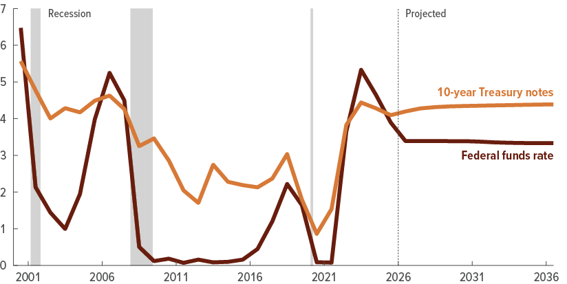
After a period of aggressive rate increases between 2022 and 2023 to curb high inflation, the Fed maintained elevated rates in 2024 and early 2025 as inflation pressures remained above target. By the start of 2026, with inflation showing signs of easing but still above the Fed’s 2% goal, the Federal Funds Rate target range settled at 3.50%–3.75%.

This higher rate environment reflects the Fed’s ongoing effort to balance price stability with labor market strength.

Quick Comparison: Past Rate Cycles

Period	Target Rate	Economic Context
2008 (Financial Crisis)	Near 0%	Emergency easing
2018	2.25% – 2.50%	Pre-pandemic tightening
2020 (Pandemic)	0% – 0.25%	Crisis response
2023–2025	4.25% – 5.25%	Inflation fight
2026	3.50% – 3.75%	Easing stabilization

(Actual rates and ranges sourced from Federal Reserve historical releases and FRED.)

The Federal Funds Rate is the bedrock of U.S. monetary policy — and understanding it is essential to interpreting interest rates, financial markets, and economic cycles. It tells readers not only what the Fed is targeting but why those targets matter for everyday financial decisions.

2.2 How the FOMC Decides on Rate Hikes or Cuts

The Federal Open Market Committee (FOMC) does not adjust interest rates at random. Every change — whether a hike, a cut, or holding steady — is the outcome of a deliberate, scheduled process that incorporates economic data, projections, and forward guidance. Understanding this process gives readers a clear view of why the Federal Reserve acts when it does.

Meeting Schedule — 8 Times per Year

The FOMC meets regularly to review economic conditions and decide whether to adjust monetary policy. These meetings occur eight times per year on a pre-announced schedule, typically every six to eight weeks.

For 2026, the FOMC meeting calendar is:

Meeting	Dates (Tentative / Official)
1	January 27–28, 2026
2	March 17–18, 2026
3	April 28–29, 2026
4	June 9–10, 2026
5	July 28–29, 2026
6	September 22–23, 2026
7	November 3–4, 2026
8	December 15–16, 2026

(Source: Federal Reserve official FOMC calendar)

At each meeting, policymakers assess inflation data, labor market metrics, financial conditions, global developments, and various economic forecasts. After discussion and debate, the committee votes on the policy statement and the target range for the Federal Funds Rate.

Most meetings conclude with a policy statement — explaining any changes and the reasoning behind them — and, four times per year, the Fed releases detailed economic forecasts.

Economic Projections (SEP)

One of the most important releases from the FOMC is the Summary of Economic Projections (SEP), which accompanies four meetings per year (typically in March, June, September, and December).

The SEP includes:

• GDP Growth forecasts
• Unemployment rate projections
• Inflation projections (both overall and core measures)
• Federal Funds Rate forecasts (expressed in the “dot plot”)

By providing these forecasts, the Fed offers transparency about where its voting members expect the economy to be in the near future. Investors, businesses, and economists use the SEP to anticipate future rate moves based on evolving economic conditions.

For example, the December 2025 SEP showed a median projection that many Fed officials expect inflation to move closer to the 2% long-run target over the next couple of years without requiring additional aggressive rate hikes. This type of guidance influences how traders price interest rate–sensitive assets.

Dot Plot — What It Is and How to Read It

The “Dot Plot” is arguably the most widely analyzed part of the SEP.

What the Dot Plot Shows:
Each dot represents an individual FOMC participant’s view of where the Federal Funds Rate should be at the end of each calendar year and at the long-run equilibrium.

• Each participant places a dot on a chart for each year ahead.
• The median of the dots is often used as the market’s expected path of interest rates.

Why It Matters:
The Dot Plot translates policymakers’ expectations into a visual forecast. Unlike a formal policy decision, it reflects opinions about where rates should go under current economic conditions.

For example:

• If many dots cluster above the current rate, it suggests the committee expects future rate hikes.
• If most dots cluster below, it suggests future rate cuts.
• A mostly horizontal cluster suggests rates may remain steady.

2025–2026 Dot Plot Insight:
In the most recent Dot Plot, the median projection indicated that many policymakers expect the Federal Funds Rate to stay near current levels through 2026, with gradual adjustments dependent on incoming economic data — especially inflation and labor market trends.

This doesn’t guarantee future decisions, but it offers guidance on how policymakers think about the future path of rates.

Putting It All Together

Here’s how the decision process unfolds:

1. Before the Meeting:
   • Staff economists and regional Fed banks prepare detailed economic reports.
   • The Beige Book — a compilation of regional economic conditions — is distributed.
   • FOMC members review inflation, GDP growth, jobs, and financial stability data.
2. During the Meeting:
   • Policymakers discuss economic conditions and downside/upside risks.
   • They debate whether the data support hiking, cutting, or holding rates.
   • They consider global economic developments (e.g., energy prices, trade policy, financial stress).
3. Decision and Communication:
   • The policy statement is released, outlining the decision and economic reasoning.
   • Four times per year, the SEP and Dot Plot accompany the statement.
   • The Fed Chair holds a press conference to explain the decision.

Why This Matters for Markets and Businesses

Every part of this process — from the meeting schedule to the Dot Plot — influences expectations in financial markets:

• Stock markets react to perceived future rate paths.
• Bond markets adjust yields based on expected interest rates.
• Currency markets (USD) move with global rate differentials.
• Businesses and consumers adapt plans based on economic guidance.

By understanding how the FOMC decides on rate hikes or cuts, your readers will better interpret Fed decisions and anticipate their impact on borrowing costs, investment decisions, and economic growth.

2.3 Rate Hikes vs Rate Cuts: What They Signal

One of the most important ways the Federal Reserve communicates its views on the economy is through changes in the Federal Funds Rate. When the Federal Open Market Committee (FOMC) raises or cuts rates, it is signaling its assessment of economic conditions — particularly inflation, job markets, and financial stability.

Below is a detailed explanation of what rate hikes and cuts typically signal, why they are used, and how real economic data supports these interpretations.

Inflation Control — Why Rate Hikes Are Used

Rate hikes — increases in the Federal Funds Rate — are primarily used when inflation is rising faster than the Federal Reserve considers healthy for the economy.

What Higher Rates Do

When the Fed raises interest rates:

• Borrowing becomes more expensive for consumers and businesses
• Consumer spending slows (e.g., fewer big-ticket purchases like homes and cars)
• Business investment slows due to higher loan costs
• Demand in the economy decreases, which reduces price pressures

Higher interest rates generally cool economic activity, which in turn helps control rising prices.

Real Data: Inflation Context

For much of 2022–2024, the U.S. experienced inflation well above the Federal Reserve’s 2% target. At its peak in mid-2022:

• CPI inflation reached 9.1% year-over-year (June 2022)
• Core CPI (excluding food and energy) topped 6.0%+
  These elevated inflation rates prompted the Fed to raise rates aggressively, moving the Federal Funds Rate from near 0% in early 2022 to a range above 5.00% by early 2023.

By late 2025 and early 2026:

• PCE inflation eased but remained above target at ~2.8% y/y, showing inflation pressures were still present but moderating.
• Core inflation measures similarly stayed above 2%.

Rate hikes in this environment signaled the Fed’s commitment to controlling inflation even as prices began to slow. Markets interpreted these hikes as necessary to anchor inflation expectations.

Signal Summary:
Rate hikes signal the Fed is prioritizing inflation control.

Economic Slowdown Support — Why Rate Cuts Are Used

Interest rate cuts — reductions in the Federal Funds Rate — are used when economic growth slows significantly, unemployment rises, or financial stress threatens broader economic activity.

What Lower Rates Do

When the Fed cuts interest rates:

• Borrowing becomes cheaper (encourages consumer and business loans)
• Mortgage and auto loan rates typically fall
• Investment becomes more attractive
• Liquidity increases in financial markets

These conditions support economic activity by making credit more accessible and affordable.

Real Data: Growth and Slowdown Indicators

Economic slowdowns often feature:

• Declining GDP growth
• Rising unemployment
• Falling consumer spending

During the 2008 financial crisis, the Fed quickly cut rates to near 0% to combat severe contraction.
Similarly, in March 2020, the Fed cut rates aggressively as COVID-19 economic shutdowns stalled growth, bringing the Federal Funds Rate down to the 0%–0.25% range.

Signal Summary:
Rate cuts signal the Fed is trying to support the economy amid slowing growth or recession risks.

Financial Stability Concerns — The Third Signal

In addition to inflation and growth, rate decisions can also reflect concerns about financial stability — that is, the health and smooth functioning of financial markets.

Elevated Financial Risk

Sometimes the Fed may adjust policy not strictly because of inflation or GDP data, but to prevent or respond to market disruptions.

For example:

• Market volatility spikes (e.g., stock markets plunging)
• Credit markets freeze (banks reluctant to lend)
• Liquidity dries up in key markets

During the 2008 crisis and in the early pandemic period, the Fed didn’t just cut rates — it took extraordinary measures (like quantitative easing and emergency lending) to stabilize markets.

Rate decisions in this context signal that policymakers are concerned about instability that could spill over into the real economy.

Signal Summary:
Policy moves due to financial stability concerns indicate the Fed is acting to prevent systemic risk.

Putting It All Together — Signals and Market Interpretation

Policy Action	Primary Signal	Typical Economic Context
Rate Hikes	Inflation control	Rising prices above target
Rate Cuts	Economic support	Slowing growth, recession risk
Policy Adjustments for Stability	Financial market health	Market stress, liquidity concerns

Market Reaction to These Signals

Financial markets interpret Fed policy not just on the basis of the rate level, but on what the rate signal suggests about future economic conditions:

• Equities tend to perform better when rate cuts are anticipated because cheaper borrowing supports corporate earnings.
• Bonds may rally (yields fall) when cuts are expected.
• The U.S. dollar often strengthens on rate hikes (higher rates attract foreign capital) and weakens on cuts.

2.4 Historical Interest Rate Cycles (Data Section)

To understand why the Federal Reserve sets interest rates where it does today, it helps to look back at key historical cycles where monetary policy played a pivotal role in steering the U.S. economy. Below are four major monetary policy eras, with real data showing how aggressively the Fed responded to economic conditions.

1. 1980s Inflation Fight

In the late 1970s and early 1980s, the United States faced double-digit inflation, eroding purchasing power and undermining economic stability. To bring inflation under control, the Fed — led by Chairman Paul Volcker — raised the Federal Funds Rate to historically high levels.

Key Facts:

• Peak Federal Funds Rate: ~20% (June 1981)
• Inflation (CPI) exceeded 13% in 1979–1980
• The high interest rates led to two short recessions (1980 and 1981–1982), but successfully broke the back of runaway inflation.

This period is the gold standard for a dramatic inflation-fighting strategy. By accepting short-term economic pain (recessions), the Fed restored price stability that underpinned long-term growth.

2. 2008 Financial Crisis

The global financial crisis of 2007–2008 led to one of the most severe economic downturns since the Great Depression. Mortgage defaults, bank failures, and collapsing markets pushed the Federal Reserve to slash interest rates and introduce unconventional policy tools.

Key Facts:

• Peak Federal Funds Rate prior to crisis: 5.25% (mid-2007)
• Fed cut to 0.00%–0.25% by December 2008
• Introduced Quantitative Easing (QE) — large-scale asset purchases of Treasury and mortgage-backed securities.

The near-zero rate policy stayed in place for several years as the Fed worked to support a fragile recovery. This era marked the beginning of unconventional central bank tools in modern monetary policy.

3. 2020 Pandemic Response

As COVID-19 spread in early 2020, economic activity plunged due to lockdowns, job losses, and supply disruptions.

The Fed acted quickly to cushion the blow.

Key Facts:

• Federal Funds Rate cut from 1.75% to 0.00%–0.25% in March 2020
• Unemployment spiked to 14.8% in April 2020 (the highest since the Great Depression)
• Fed launched massive QE programs, purchasing trillions of dollars in Treasury and mortgage-backed securities to support liquidity.

This response helped stabilize markets and provided breathing room for fiscal stimulus to work.

4. 2022–2024 Inflation Tightening Cycle

Following the pandemic, supply chain disruptions, fiscal stimulus, and strong consumer demand pushed inflation well above target.

From early 2022, the Federal Reserve began one of the most aggressive rate-hike cycles in decades to quell inflation.

Key Facts:

• Federal Funds Rate (start of 2022): 0.00%–0.25%
• Peak Federal Funds Rate (2023–2024): 5.25%–5.50%
• Inflation (CPI) hit 9.1% year-over-year in June 2022, the highest in 40 years
• By late 2025, inflation had eased but remained above target (PCE ~2.8%)

This tightening cycle was designed to slow demand, re-anchor inflation expectations, and bring price growth closer to the Fed’s 2% goal.

Comparing Peak Federal Funds Rates by Cycle

For easy comparison, use the following table to show how dramatic rate shifts have been across major economic cycles:

Policy Cycle	Peak Federal Funds Rate	Reason for Policy Action	Outcome / Context
1980s Inflation Fight	~20% (1981)	Break double-digit inflation	Inflation fell; deep recessions
Pre-2008 / Financial Crisis	5.25% (2007)	Normal monetary stance pre-crisis	Crisis triggered near-zero cuts
2008 Crisis & Recovery	0.00%–0.25% (2008–2015)	Combat financial meltdown	Supported recovery, low rates persisted
2020 Pandemic Response	0.00%–0.25% (2020)	Halt economic collapse	QE + fiscal support
2022–2024 Tightening Cycle	5.25%–5.50%	Fight post-pandemic inflation	Inflation fell towards target

What This Tells Us

• 1980s: High-rate discipline was necessary to restore price stability.
• 2008: Zero rates and QE were needed to prevent systemic collapse.
• 2020: Swift easing stabilized markets during unprecedented shutdowns.
• 2022–2024: A rapid rate-hiking cycle was employed to manage inflation.

These historical comparisons help readers understand that interest rate policy is not static — it adapts to the greatest economic challenges of each era. Using real data clarifies the trends and reinforces why the Fed’s current policy stance matters.

2.5 Real Interest Rates vs Nominal Rates

When discussing interest rates, economists and policymakers distinguish between nominal rates and real rates.
Understanding this distinction is essential because real interest rates reflect the true cost of borrowing after adjusting for inflation, which is often more meaningful for businesses, consumers, and investors.

1. Nominal Interest Rates — The Face Value

Nominal interest rates are the rates you see quoted publicly — such as the Federal Funds Rate, mortgage rates, or bond yields. These rates do not account for inflation.

For example:

• The current Federal Funds Rate target range in 2026 is 3.50%–3.75%.
• A 30-year fixed mortgage rate might be around 6.5%–7% (varies weekly with market conditions).

These are nominal figures — the stated rates without adjustment for the changing value of money over time.

2. Real Interest Rates — Adjusting for Inflation

Real interest rates are calculated by subtracting inflation from nominal interest rates. This tells you the true purchasing power cost of borrowing or the actual return on an investment after inflation erodes value.

Formula:

Real Interest Rate = Nominal Interest Rate − Inflation Rate

Example with Real Data (2026 Context):

• Nominal Federal Funds Rate (mid-2026): ~3.60%
• Inflation (PCE, Fed’s preferred measure): ~2.8%
• Real Fed Funds Rate ≈ 3.60% − 2.80% = 0.80%

This means that after adjusting for inflation, the actual cost of holding cash or short-term assets is closer to 0.8% in real terms, not the 3.6% face value.

3. Why Real Rates Matter More Than Nominal Rates

Real rates offer a clearer picture of monetary policy’s stance and its effect on economic behavior:

A. True Cost of Borrowing

Borrowers make decisions based on real costs.
If inflation is high, even moderately high nominal rates may feel cheap in real terms.

Example:

• A business may view a nominal rate of 6.5% on a loan as expensive — but if inflation is 4%, the real rate is just 2.5%, which might still encourage investment.

B. Investment Decisions

Investors look at real returns to evaluate whether an investment actually earns money above inflation.

Example:

• A bond yielding 5% with inflation at 3% generates a real return of 2%.

C. Monetary Policy Implications

Central bankers focus heavily on real rates because they reflect the tightness or ease of monetary policy.

• When real rates are positive and rising, monetary policy is relatively tight — borrowing is expensive in inflation-adjusted terms.
• When real rates are negative or low, monetary policy is accommodative — encouraging borrowing and spending.

D. Economic Growth and Savings Behavior

Real rates influence savings vs. spending decisions:

• Higher real rates encourage saving and reduce spending.
• Lower or negative real rates discourage saving and stimulate consumption.

4. Historical Real Rate Context

Looking at real rates over time helps illustrate economic cycles:

Era	Nominal Rate (Fed Funds)	Inflation Rate	Real Rate
1981 Inflation Fight	~20%	~12%	~8%
2008 Crisis Era	0.25%	~3%	−2.75%
2020 Pandemic	0.25%	~1.4%	−1.15%
2026 Context	~3.60%	~2.8%	~0.80%

This table shows:

• Real rates were extremely high in the early 1980s — a deliberate choice to combat severe inflation.
• During crisis periods (2008, 2020), real rates were negative, stimulating economic activity by making borrowing cheap in inflation-adjusted terms.
• In 2026, real rates are positive but relatively moderate — signaling a balanced stance where inflation is being addressed without excessively tightening financial conditions.

3. Why the Fed Changes Policy (Economic Reasoning Behind Decisions)

3.1 Controlling Inflation

Inflation — the general rise in prices of goods and services over time — is one of the Federal Reserve’s most important policy targets. The Federal Reserve aims for a long-run inflation rate of 2 percent, a level seen as consistent with price stability and sustainable economic growth. To understand how the Fed fights inflation, it’s critical to explore what causes inflation, the difference between headline and core measures, and why inflation expectations matter.

Causes of Inflation: Demand vs. Supply

Inflation can be driven by two broad forces: demand-pull and cost-push (supply-side) inflation.

1. Demand-Pull Inflation
Demand-pull inflation occurs when aggregate demand in the economy outpaces aggregate supply. Simply put, when consumers, businesses, and governments want more goods and services than the economy can produce at full capacity, prices rise.

Examples of demand-pull drivers:

• Strong consumer spending
• Government fiscal stimulus
• Filling labor shortages
• Rapid credit growth

Real Data Context:
In 2021–2022, the U.S. economy experienced unusually strong demand as:

• COVID-19 restrictions eased
• Fiscal stimulus packages exceeded $5 trillion combined
• Consumer spending rebounded rapidly
  This surge in demand contributed to high inflation, with CPI hitting 9.1% year-over-year in June 2022 — the highest in over 40 years.

2. Cost-Push (Supply-Side) Inflation
Cost-push inflation happens when the cost of production rises, and producers pass that cost onto consumers. These pressures can come from:

• Rising energy prices
• Supply chain bottlenecks
• Labor shortages
• Import price increases (tariffs, exchange rate shifts)

Real Data Context:
In 2021–2022, global supply chain disruptions, semiconductor shortages, and elevated shipping costs contributed to price pressures even as supply struggled to keep up with demand.

Core vs. Headline Inflation

Understanding the difference between core and headline inflation helps explain how policymakers interpret price pressures.

Headline Inflation
This measures the overall rate of inflation, including all consumer prices — food, energy, housing, transportation, medical care, and more.

• Headline inflation can be volatile because energy and food prices move frequently.
• For example, a sudden spike in gasoline prices can push headline CPI higher even if other prices are stable.

Core Inflation
Core inflation excludes food and energy because their prices often fluctuate due to short-term supply shocks unrelated to broader economic trends.

Why this matters:

• Core inflation offers a clearer view of underlying inflation pressures.
• Policymakers watch core measures to distinguish between temporary price movements and systemic inflation.

Real Data Comparison (Dec 2025)

• Headline CPI: ~3.4% y/y
• Core CPI: ~3.7% y/y
  This indicates that even after removing volatile food and energy costs, underlying price pressures remained robust.

Inflation Expectations

Inflation expectations are how households, businesses, and markets anticipate future inflation. These expectations influence real economic behavior:

• If consumers expect prices to rise faster, they may spend more today, increasing demand and fueling further inflation.
• If businesses expect higher input costs, they may raise prices pre-emptively.

The Federal Reserve pays close attention to inflation expectations as a leading indicator:

Market-Based Measures:
5-Year, 5-Year Forward Inflation Expectation Rate (derived from Treasury Inflation-Protected Securities – TIPS)

• Recently, this measure has hovered near 2.3%–2.4%, indicating markets expect inflation to moderate close to the Fed’s long-run target.

Survey Measures:
University of Michigan Consumer Sentiment Survey tracks consumer inflation expectations:

• 1-year expectations have varied between 3%–4%, signaling that households still anticipate above-target inflation in the short run.

Stable expectations near the Fed’s 2% target help anchor inflation over the long term because they reduce the incentive for wage–price spirals and aggressive pricing behavior.

Why the Fed Focuses on Inflation

When inflation is persistently above target (e.g., >3% for multiple months), it signals that price pressures may be broadening beyond temporary factors. To address this, the Fed may raise interest rates or tighten monetary conditions to cool economic activity.

Conversely, if inflation falls significantly below the 2% target, it may signal weak demand and potential slow-growth conditions, prompting policy easing.

Real Impact on Policy Decisions

For example:

• 2021–2022: Inflation surged due to demand-pull conditions and supply disruptions. The Fed responded by raising interest rates rapidly to cool demand and slow price increases.
• 2025–2026: Inflation moderated, but core inflation remained above target, signaling underlying pressures that have yet to fully dissipate. This has encouraged policymakers to maintain a cautious stance on rate cuts.

Key Takeaways

• Demand-pull inflation comes from too much demand chasing too few goods.
• Supply-side inflation arises when production costs rise.
• Headline inflation captures all price changes, while core inflation strips out volatile food and energy prices for a more stable trend.
• Inflation expectations shape consumer and business behavior — and influence monetary policy itself.

Understanding these dynamics helps readers grasp why the Fed acts aggressively during inflationary spikes and what metrics it uses to judge whether inflation is temporary or entrenched.

3.2 Preventing Recession

One of the Federal Reserve’s secondary goals is to sustain economic growth and prevent or soften recessions. A recession — a significant decline in economic activity lasting months or more — can trigger rising unemployment, falling incomes, weaker corporate profits, and financial stress. To avoid severe downturns, the Fed watches several leading economic indicators that tend to signal weakening growth before it appears in headline GDP numbers.

Below are the primary indicators the Fed uses — along with current or recent data — to assess recession risk.

Leading Indicators of Economic Slowdown

Leading indicators are economic variables that tend to change before the overall economy begins to contract. They give policymakers and investors early warning signals.

Key leading indicators include:

• Yield Curve
• Consumer Spending Trends
• Business Investment
• Manufacturing Activity
• Labor Market Signals

Among these, two of the most closely watched by the Federal Reserve are yield curve inversion and consumer spending patterns.

Yield Curve Inversion — A Classic Warning Sign

The yield curve plots interest rates across different maturities of U.S. Treasury securities — from short-term bills to long-term bonds.

When the curve is normal, long-term rates are higher than short-term rates. This reflects expectations that the economy will grow and inflation will rise over time.

However, when the yield curve inverts, short-term rates exceed long-term rates — signaling that investors expect weaker growth in the future.

Why It Matters:
Yield curve inversions have historically preceded recessions — sometimes by 6–24 months — making them one of the most reliable recession predictors.

Recent Data (2025–2026):

• In early 2025, the 2-year Treasury yield exceeded the 10-year Treasury yield, creating a slightly inverted yield curve.
• As of late 2025, the 2-year yield traded above the 10-year yield by a narrow margin, suggesting market expectations of slower growth ahead.

For example:

• 2-Year Treasury Yield: ~4.50%
• 10-Year Treasury Yield: ~4.30%
• This inversion reflects investor caution about future growth.

An inverted yield curve suggests that markets are pricing in lower growth or future rate cuts, often before economic data confirms a slowdown.

Consumer Spending Slowdown — A Key Demand Signal

Consumer spending accounts for roughly two-thirds of U.S. Gross Domestic Product (GDP). When consumers slow down on spending — particularly on big-ticket items — it often signals weakening confidence and slower economic growth.

The Fed monitors consumer spending through trends in retail sales, disposable income, credit usage, and service sector activity.

Recent Consumer Spending Trends (2025):

• Retail sales have continued to grow, but at a moderating pace compared with the post-pandemic rebound.
• Recent monthly data showed retail sales growth slowing to around 0.3%–0.4% per month, below the stronger pace seen in earlier economic expansions.

Slower consumer spending growth can indicate that households are becoming cautious — potentially due to higher borrowing costs, inflation pressures, or labor market uncertainty.

Other Leading Indicators the Fed Watches

While yield curve inversion and consumer spending are critical signals, the Fed also watches:

• Manufacturing data (PMI / ISM indices) — contraction can signal broader economic weakness
• Business investment levels — lower investment suggests cautious business confidence
• Jobless claims — increases in weekly unemployment claims can precede broader layoffs
• Building permits and housing starts — a cooling housing market signals weaker economic activity

For example, if the ISM Manufacturing PMI falls below 50, it indicates contraction — a warning bell for broader economic slowdown.

How the Fed Responds to Recession Risks

When multiple leading indicators turn negative, the Federal Reserve may:

• Cut interest rates to make borrowing cheaper
• Increase liquidity in financial markets
• Lower reserve requirements for banks
• Use forward guidance to assure markets of policy support

Rate cuts reduce borrowing costs, stimulate consumer and business spending, and cushion economic slowdowns.

For instance, during the 2020 COVID-19 recession, the Fed cut the Federal Funds Rate to 0.00%–0.25% and implemented large-scale asset purchases to support financial markets and credit flows.

Similarly, during the 2008 Financial Crisis, sharp rate cuts were used in conjunction with quantitative easing to combat severe contraction.

What Recession Signals Tell Policymakers

Indicator	Signal	Why It Matters
Yield Curve Inversion	The market expects slower growth	Historically precedes recessions
Consumer Spending Slowdown	Falling demand	Reduced GDP growth impact
Manufacturing Contraction	Lower output	Signals broader economic weakness
Rising Unemployment Claims	Labor market weakening	The market expects slower growth

3.3 Stabilizing the Financial System

One of the less-visible but critically important responsibilities of the Federal Reserve System is maintaining financial stability. Beyond inflation and employment goals, the Fed must ensure that the U.S. financial system operates smoothly — especially during times of stress. When markets seize up or banks face solvency pressures, the Fed acts to prevent a localized problem from cascading into a full-blown crisis.

Below are the main ways the Fed intervenes when financial stability is threatened: banking stress monitoring, liquidity support, and emergency lending programs — explained with real examples and recent data.

Banking Stress: What It Is and How the Fed Monitors It

Banking stress refers to periods when financial institutions face solvency or liquidity pressure. It can show up as:

• Rising non-performing loans on bank balance sheets
• Sharply declining bank stock prices
• Credit markets tightening
• Deposit outflows

A key measure of banking stress is the Senior Loan Officer Opinion Survey (SLOOS) published by the Federal Reserve. When banks tighten lending standards, it signals they perceive more risk in the economy. During periods of stress, this tightening shows up before broader economic data deteriorates.

Real Example — 2023 Regional Bank Stress:
In early 2023, several U.S. regional banks faced stress after sharp losses on interest-rate-sensitive assets and deposit withdrawals. This triggered concerns about bank liquidity and prompted risk repricing in credit markets. The Fed and federal regulators closely monitored bank stress indicators and coordinated responses to prevent contagion.

Liquidity Crises: When Markets Dry Up

A liquidity crisis occurs when there isn’t enough cash or readily sellable assets in financial markets — even if institutions are fundamentally solvent. Without liquidity, markets stop functioning efficiently, and prices can move violently.

Liquidity freeze‐ups can occur in:

• Government bond markets
• Corporate credit markets
• Money markets
• Repo markets (overnight lending between financial firms)

Real Example — March 2020:
At the onset of the COVID-19 pandemic, liquidity in U.S. Treasury markets and funding markets deteriorated sharply. Investors rushed to sell assets and hoard cash. Spreads widened dramatically, and benchmark yields became erratic.

To stabilize liquidity, the Federal Reserve announced multiple liquidity facilities and expanded open market operations to inject cash directly into markets.

Emergency Lending Programs: Crisis Tools in Action

When standard policy tools (e.g., interest rates) aren’t enough, the Fed can implement emergency lending programs to support specific markets or institutions. These facilities often operate temporarily under Section 13(3) of the Federal Reserve Act.

Here are several significant examples:

1. 2008 Financial Crisis Programs

During the 2008 crisis, the Fed launched multiple emergency facilities, including:

• Term Auction Facility (TAF) — to enhance liquidity to banks
• Primary Dealer Credit Facility (PDCF) — lending to dealers that buy/sell government securities
• Commercial Paper Funding Facility (CPFF) — supporting short-term corporate debt markets
• Term Asset-Backed Securities Loan Facility (TALF) — boosting consumer and business credit markets

Data in Context:
At the peak of these programs, the Fed expanded its balance sheet from about $900 billion pre-crisis to over $2 trillion by 2009 as liquidity programs and asset purchases grew.

2. 2020 Pandemic Response — Broad Liquidity Measures

When COVID-19-stricken markets in March 2020, the Fed acted rapidly:

• Cut the Federal Funds Rate to 0.00%–0.25%
• Massive QE (asset purchases) totaling trillions
• Money Market Mutual Fund Liquidity Facility (MMLF)
• Primary Market Corporate Credit Facility (PMCCF)
• Secondary Market Corporate Credit Facility (SMCCF)
• Paycheck Protection Program Liquidity Facility (PPPLF)

These programs ensured credit markets — from corporate bonds to small business lending — continued functioning even as economic activity contracted sharply.

By June 2020, the Fed’s balance sheet had nearly doubled, reaching approximately $7 trillion — reflecting massive emergency liquidity injections.

3. 2023–2024 Regional Bank Support Mechanisms

In response to stress at some regional banks in 2023, the Fed provided a Bank Term Funding Program (BTFP):

• Banks could pledge high-quality securities at par value for liquidity
• This prevented forced asset sales at losses
• Helped stabilize confidence in the banking system

The BTFP helped slow deposit outflows and ease market stress without requiring public bailouts.

How These Tools Keep the Financial System Stable

The Federal Reserve serves as the “lender of last resort.” When financial stress intensifies:

1. Standard policy tools (rate changes) may be insufficient
2. Liquidity injections via open market operations supply cash to financial institutions
3. Emergency lending facilities provide direct support to markets that are frozen or dysfunctional

This prevents short-term liquidity problems from turning into systemic failures — as happened during the Great Depression.

Why This Matters for the Broader Economy

If banking stress and liquidity crises are left unaddressed:

• Credit flows to households and businesses dry up
• Markets lose confidence
• Economic contraction accelerates
• Unemployment rises

By stabilizing the financial system, the Fed supports:

• Smooth functioning of payment systems
• Access to credit for consumers and businesses
• Confidence in financial markets

Key Takeaways

• The Fed monitors bank stress indicators to detect early signs of financial instability.
• When markets seize up, the Fed supplies liquidity to keep financial plumbing working.
• In the most severe conditions, the Fed activates emergency lending facilities to support credit markets and financial institutions.

3.4 Managing Employment Levels

The Federal Reserve’s mandate includes maximum sustainable employment — meaning the highest level of job creation and participation the economy can sustain without fueling excessive inflation. To assess labor market conditions, policymakers examine several high-frequency labor indicators. These data help the Fed decide whether to tighten or ease monetary policy.

Below are the most important employment metrics the Fed watches — with recent data to give readers real context.

Nonfarm Payroll Data — Measuring Job Growth

Nonfarm payrolls represent the total number of jobs added or lost across the U.S. economy, excluding farm workers, private household employees, and non-profit organization workers. This monthly statistic — released by the Bureau of Labor Statistics (BLS) — is one of the most important signals of labor market strength.

Why It Matters

• Strong payroll gains signal employers are confident and expanding.
• Weak or negative payroll growth may indicate an economic slowdown.

Recent Data (January 2026)

• U.S. nonfarm payrolls increased by +182,000 jobs in January 2026.
  This reflects continued job growth, though at a more moderate pace than earlier post-pandemic expansions.

A sustained slowdown in job gains over several months would signal weakening labor demand and could prompt the Fed to consider rate cuts to support jobs and overall economic activity.

Labor Force Participation Rate — Capturing Worker Engagement

The labor force participation rate measures the share of the working-age population that is either employed or actively looking for work. This metric goes beyond unemployment because it includes individuals who left the labor force.

Why It Matters

• A higher participation rate suggests confidence in job opportunities.
• A declining participation rate may indicate discouragement or structural labor issues.

Recent Data

• As of January 2026, the labor force participation rate was approximately 62.6% — below the pre-pandemic level (around 63.4% in early 2020).

This suggests that while job creation remains solid, a portion of the working-age population remains out of the labor force. The Fed watches this closely because rising participation can put additional pressure on wage growth and inflation if the labor market tightens further.

Job Openings and Labor Turnover Survey (JOLTS)

The JOLTS report measures job openings, hires, and separations each month. This dataset provides deeper insight into the demand side of the labor market.

Why JOLTS Matters

• A high number of job openings indicates strong labor demand.
• A decline in openings may signal weakening employer confidence and slower hiring ahead.

Recent JOLTS Data (Late 2025)

• Total U.S. job openings remained elevated, with millions of positions available across industries.
  While the absolute numbers can fluctuate monthly, elevated openings indicate that employers are still seeking workers — a sign of ongoing labor demand.

However, if job openings begin to trend downward — especially alongside slower job growth — the Fed watches this as a potential early sign of labor market easing.

Why These Employment Indicators Matter for Monetary Policy

The Fed does not set interest rates based solely on one statistic. Instead, it evaluates a composite view of labor conditions:

• Consistent job growth suggests a healthy economy that may tolerate tighter policy.
• High labor force participation can signal a robust labor market with rising wage pressures.
• Elevated job openings reflect strong demand for workers, which can push wages up and fuel inflation.

When the labor market overheats — with low unemployment, high job openings, and rising wages — it can contribute to inflationary pressures. In such cases, the Fed may raise rates to slow economic demand. Conversely, if job growth weakens and openings decrease, the Fed may consider rate cuts to support economic activity.

Employment Data Summary (Recent Figures)

Indicator	Latest Value	Pre-Pandemic Level	Trend Implication
Nonfarm Payroll Growth	+182,000 (Jan 2026)	N/A	Continued job growth
Labor Force Participation Rate	62.6%	~63.4% (2020)	Lower participation than pre-pandemic
Job Openings (JOLTS)	Elevated	Elevated	Strong labor demand

Core Insight

Understanding labor market health gives readers insight into why the Fed maintains certain policy stances. Strong employment numbers — even during periods of above-target inflation — can justify continued rate hikes or a pause rather than cuts. Weakening labor data, on the other hand, can signal recession risk and move the Fed toward easing.

This employment perspective solidifies how the Fed balances its dual mandate — aiming for price stability while ensuring robust job markets.

4. How Federal Reserve Policy Affects Small Businesses

Federal Reserve policy does not just affect Wall Street — it directly influences how small businesses borrow, manage cash flow, hire employees, and plan expansion. When the Federal Funds Rate changes, it moves through the banking system and alters loan rates, credit availability, and overall demand conditions. With the Federal Funds Rate currently in the 3.50%–3.75% range after peaking above 5% during the 2022–2024 inflation fight, borrowing conditions remain tighter than pre-pandemic levels. That environment significantly impacts small business operations.

4.1 Borrowing Costs and Business Loans

When the Federal Reserve raises or lowers interest rates, small business financing costs move accordingly. Most small business loans are tied directly or indirectly to benchmark rates such as the prime rate, which typically moves in line with the Federal Funds Rate.

• SBA Loans

Small Business Administration (SBA) loans, especially the popular 7(a) loan program, often carry variable interest rates tied to the prime rate. For example, when the Fed raised rates aggressively between 2022 and 2023, the prime rate climbed above 8%. That meant SBA loan rates for many borrowers moved into the 9%–11% range, depending on terms. For a $500,000 SBA loan: At 6% interest, the annual interest cost ≈ $30,000. At 10% interest, the annual interest cost ≈ $50,000. That $20,000 difference directly affects profitability and reinvestment capacity.

• Variable-Rate Credit Lines

Many small businesses rely on revolving credit lines for working capital. These are typically variable-rate loans tied to the prime rate or SOFR. When rates rise: Monthly interest payments increase immediately. Cash flow becomes tighter. Businesses may reduce inventory purchases or delay expansion. When rates fall: Credit becomes cheaper. Short-term financing costs decline. Businesses can manage seasonal cycles more easily.

• Commercial Real Estate Loans

Commercial real estate (CRE) loans are highly sensitive to interest rate movements. Between 2022 and 2024: CRE financing costs rose sharply. Property valuations declined due to higher discount rates. Refinancing became more expensive. For small businesses owning retail space, office property, or warehouses, higher rates increase: Mortgage payments, refinancing risks, and debt-service coverage pressures

4.2 Cash Flow and Working Capital

Interest rate policy influences not just borrowing costs but also daily operational liquidity.

• Interest Expense Modeling Example

Assume a small manufacturing company carries $1 million in floating-rate debt. At 5% interest: Annual interest expense = $50,000. At 8% interest: Annual interest expense = $80,000. That additional $30,000 must come from: Reduced profit margins, higher prices to customers, or cost cuts elsewhere. In high-rate environments, businesses must actively model interest sensitivity scenarios to protect margins.

• Margin Compression Analysis

When borrowing costs rise while input prices remain elevated (e.g., energy, wages), margins compress. Example: Revenue growth slows to 3%. Wage growth remains around 4%. Interest expenses rise 20–30.% This squeeze forces businesses to: Raise prices (risking customer demand), Reduce staff, and Delay capital investments.

4.3 Hiring Decisions

Federal Reserve policy affects labor markets indirectly through financing conditions and demand strength.

• Wage Cost Impact

As of early 2026, Average hourly earnings are growing around 4% year-over-year. The unemployment rate is approximately 4.3%. In tighter labor markets, Wage pressures increase. Small businesses must offer higher pay to attract workers. Payroll expenses grow faster than revenue during slowdowns. Higher interest rates can reduce demand, leading businesses to freeze hiring or reduce staff growth.

• Expansion vs. Contraction Planning

When rates are low, Businesses expand locations. Invest in equipment. Hire additional staff. When rates are high, Expansion plans slow. Capital expenditures decline. Hiring decisions become cautious. Small businesses must align their expansion strategy with credit cycle conditions.

4.4 Industry-Specific Impact

Federal Reserve policy affects industries differently depending on capital intensity and sensitivity to consumer demand.

• Manufacturing

Manufacturing is capital-intensive. Higher rates increase equipment financing costs and reduce demand for durable goods. During tightening cycles, New factory expansion slows. Inventory management becomes conservative.

• Retail

Retail is highly dependent on consumer credit and disposable income. Higher rates: Increase credit card interest rates. Reduce discretionary spending. Slow large purchases. Retailers often experience margin pressure during high-rate cycles.

• Technology Startups

Startups rely heavily on venture capital and debt financing. When rates rise, Venture funding tightens. Valuations decline. Growth-at-all-cost models become less viable. Higher real interest rates reduce investor appetite for speculative growth companies.

• Real Estate Developers

Real estate is one of the most rate-sensitive sectors. Higher rates: Increase mortgage and development financing costs. Reduce buyer affordability. Lower property valuations. Between 2022 and 2024, commercial real estate faced valuation pressure as financing costs surged. Final Insight for Small Business Owners: Federal Reserve policy directly shapes: Loan affordability, hiring confidence Expansion timing Profit margins Industry competitiveness. Understanding where the Fed stands in the interest rate cycle allows small businesses to plan strategically — whether that means refinancing debt, delaying expansion, conserving cash, or accelerating investment before rates rise again.

5. How Federal Reserve Policy Affects Consumers

Federal Reserve policy directly influences household finances. When the Fed raises or lowers the Federal Funds Rate, the effects ripple through mortgage markets, credit cards, auto loans, student loans, and savings accounts. For consumers, this determines how expensive it is to borrow — and how much they earn on savings. As of early 2026, with the Federal Funds Rate in the 3.50%–3.75% range following the 2022–2024 tightening cycle, borrowing costs remain elevated compared to the ultra-low rate period of 2020–2021. Below is how those policy shifts affect everyday Americans.

5.1 Mortgage Rates and Housing Affordability

Mortgage rates are highly sensitive to Federal Reserve policy because they move with Treasury yields, particularly the 10-year Treasury note.

• 30-Year Fixed Mortgage Trends

Mortgage rate movement over recent cycles: 2020 pandemic low: ~2.7% (historic lows) 2022–2023 tightening peak: above 7% Early 2026 average: ~6.5%–7.0% This dramatic rise from pandemic lows significantly changed housing affordability. When rates rise, Monthly mortgage payments increase sharply. Homebuyer demand cools. Housing inventory may rise. Refinancing activity declines. When rates fall, Housing demand increases. Refinancing activity accelerates. Home prices often strengthen.

• Monthly Payment Comparison Table

Example: $400,000 mortgage (30-year term) Interest Rate Monthly Payment Total Interest Over 30 Years 3% ~$1,686 ~$207,000 5% ~$2,147 ~$373,000 7% ~$2,661 ~$558,000 A move from 3% to 7% increases the monthly payment by nearly $1,000 — dramatically impacting affordability.

5.2 Credit Cards and Personal Loans

Credit card rates are directly tied to the prime rate, which moves closely with the Federal Funds Rate.

• Average APR Data

As of early 2026, the average credit card APR: ~20%–21%. Many variable-rate cards exceeded 22% during peak tightening. When the Fed raises rates, Credit card interest rises almost immediately. Carrying balances becomes significantly more expensive. For example: $5,000 balance at 15% APR → ~$750 annual interest $5,000 balance at 22% APR → ~$1,100 annual interest. That difference affects disposable income directly.

• Household Debt Levels

U.S. household debt has exceeded $17 trillion in recent Federal Reserve reports, including: Mortgage debt, Credit card balances, Auto loans, Student loans. Higher rates increase debt-servicing burdens, particularly for households carrying revolving credit.

5.3 Auto Loans and Student Loans

Auto and student loans are also influenced by interest rate policy, though student loans may be partially fixed or federally set.

• Loan Rate Comparison Chart

Recent average rates: New auto loans: ~6%–8% Used auto loans: ~8%–10% Federal undergraduate student loans (recent academic year): ~5%–6% During low-rate environments (2020–2021): Auto loan rates were often below 4%. Financing costs were significantly lower. Higher rates increase: Monthly auto payments, Total vehicle ownership costs, Student refinancing costs (for private loans)

• Delinquency Trends

Recent Federal Reserve data shows: Rising auto loan delinquency rates among subprime borrowers. Credit card delinquency rates are trending upward compared to pre-pandemic levels. Higher borrowing costs combined with elevated living expenses increase repayment pressure for many households.

5.4 Savings Accounts and CD Returns

While higher rates increase borrowing costs, they benefit savers.

• High-Yield Savings Rate Trends

In 2020, High-yield savings accounts paid below 1%. By 2024–2025: Many online banks offered 4%–5% on savings accounts. Certificates of Deposit (CDs) offered similar or slightly higher yields. Higher policy rates improve returns for: Retirees, Conservative savers, Cash-heavy households

• Real Return vs Inflation

Real return = Nominal savings rate – Inflation. Example (2026 context): Savings rate: 4.5% Inflation (PCE): ~2.8% Real return ≈ 1.7%. In contrast, during 2022 when inflation exceeded 8%: Even 2% savings rates resulted in deeply negative real returns. Thus, savers benefit most when Interest rates are high and inflation is falling.

Key Consumer Takeaways: Federal Reserve policy affects consumers through: Mortgage affordability, Credit card interest costs, Auto loan payments, Student loan refinancing, Savings yields, and Real purchasing power. When rates are high, Borrowers face tighter conditions. Savers benefit. Housing affordability declines. Credit becomes more expensive. When rates are low: Borrowing expands. Asset prices often rise. Savers earn less on deposits. Understanding these dynamics helps households make smarter decisions about refinancing, debt repayment, home buying, and savings strategies.

6. Who Benefits from Higher or Lower Interest Rates

Interest rate cycles do not affect all participants equally. When the Federal Reserve raises or lowers the Federal Funds Rate, it redistributes financial advantages across sectors of the economy. Some groups benefit from higher rates, while others thrive in low-rate environments. Understanding these shifts helps investors, businesses, and households adjust their strategy based on where the economy is in the monetary cycle.

6.1 Beneficiaries of Higher Rates

When interest rates rise, borrowing becomes more expensive — but several sectors benefit directly.

• Banks

Banks often benefit from higher rates because they earn more on loans, while deposit rates may rise more slowly. This widens the net interest margin (NIM) — the difference between what banks earn on loans and what they pay on deposits. Between 2022 and 2024, Net interest margins expanded for many large U.S. banks as loan yields increased. Higher commercial and consumer lending rates improved interest income. However, if rates rise too quickly, deposit competition increases, and credit quality can deteriorate, moderating the benefits.

• Bond Investors (New Buyers)

Higher rates allow new bond investors to lock in higher yields. Example: In 2020, 10-year Treasury yields fell below 1%. By 2023–2024, 10-year yields exceeded 4%. In early 2026, yields remain elevated compared to pandemic lows. Higher yields improve income for: Pension funds, Fixed-income investors, Insurance companies. Existing bondholders may face price declines when rates rise, but new investors benefit from higher coupon income.

• Savers

Higher rates increase returns on: Savings accounts, Certificates of Deposit (CDs), Treasury bills. High-yield savings accounts in 2024–2025 offered 4%–5%, compared to less than 1% during 2020. For retirees and conservative investors, higher nominal rates significantly improve income stability — especially when inflation is moderating.

• Money Market Funds

Money market funds invest in short-term instruments tied closely to Federal Reserve policy. As rates rose above 5% in 2023, Money market yields climbed above 5%. Assets in money market funds surged to record levels (exceeding $6 trillion in total assets in recent years). Higher policy rates directly increase money market returns, making them attractive low-risk investment vehicles.

6.2 Beneficiaries of Lower Rates

Lower interest rates stimulate borrowing, risk-taking, and investment — benefiting growth-oriented sectors.

• Growth Stocks

Growth stocks rely on future earnings projections. Lower rates reduce discount rates used in valuation models, increasing present value calculations. During the 2020–2021 near-zero rate period, Technology and high-growth stocks saw strong valuation expansion. Equity markets rallied sharply as borrowing costs fell. When rates decline, growth sectors often outperform due to cheaper capital and improved investor risk appetite.

• Real Estate Sector

Real estate is highly sensitive to interest rates. Lower mortgage rates: Increase housing affordability. Stimulate home buying. Boost property valuations. During 2020–2021, 30-year mortgage rates fell below 3%. Housing demand surged. Home prices climbed significantly. Lower rates also reduce financing costs for commercial real estate developers.

• Borrowers

Lower rates benefit consumers and businesses carrying debt. Examples: Lower mortgage payments, reduced credit card interest Cheaper business loans, and easier refinancing. Debt-heavy companies benefit significantly when rates fall.

• Venture Capital

Low interest rates encourage risk-taking and capital flows into startups. When rates are near zero: Investors seek higher returns in private markets. Venture funding expands. Startup valuations rise. Higher rates typically reduce venture funding as safer fixed-income investments become more attractive.

6.3 Sector-by-Sector Market Winners

Different sectors outperform depending on where rates are headed.

• Financials

Benefit during rising-rate environments due to improved net interest margins — provided credit quality remains stable.

• Utilities

Utilities often behave like bond proxies because they offer steady dividends. Perform better in low-rate environments. Face pressure when bond yields rise and offer competitive alternatives.

• Technology

Highly sensitive to discount rate changes. Thrive in falling-rate cycles. Face valuation compression during tightening cycles.

• Consumer Discretionary

This sector benefits when borrowing costs decline. Consumer confidence rises. Disposable income increases. Higher rates can reduce discretionary spending due to rising debt costs.

6.4 Investor Strategy Adjustments

Investors often adjust portfolios depending on the interest rate environment.

• Sector Rotation

When rates rise: Shift toward financials and value stocks. When rates fall: Shift toward growth and technology sectors.

• Duration Risk Management

Bond investors manage duration carefully: Long-duration bonds lose more value when rates rise. Short-duration bonds are less sensitive. In high-rate environments, investors often shorten bond duration to reduce volatility.

• Dividend Yield Strategy

When bond yields rise, high-dividend stocks compete directly with fixed income. Investors compare: Dividend yield vs Treasury yield, Risk premium vs bond stability. When Treasury yields exceed 4%–5%, dividend-paying equities must offer compelling growth or yield to remain attractive.

Key Insight: Interest rate cycles redistribute financial advantages. Higher rates reward savers and lenders but pressure borrowers and growth sectors. Lower rates stimulate borrowing, asset prices, and risk-taking but reduce returns for conservative investors. Understanding these dynamics helps investors align portfolios with the current phase of the Federal Reserve’s monetary cycle.

7. Who May Be Hurt by Rate Changes

While some sectors benefit from rising or falling interest rates, others face significant financial pressure. Rate increases, in particular, can expose weaknesses in heavily indebted companies, small businesses reliant on floating-rate loans, households carrying revolving credit balances, and emerging market economies dependent on U.S. dollar financing. Understanding these vulnerabilities helps readers assess risk during different phases of the monetary cycle.

7.1 Highly Leveraged Companies

Companies that rely heavily on borrowed money are among the most vulnerable when interest rates rise.

• Debt-to-Equity Ratios

A key measure of leverage is the debt-to-equity (D/E) ratio, which compares total debt to shareholder equity. A D/E ratio above 1.0 indicates more debt than equity. Highly leveraged firms (D/E above 2.0 in some industries) are especially sensitive to rising interest costs. When rates increase, Interest expense rises. Net income declines. Earnings per share fall. Credit ratings may deteriorate. Between 2022 and 2024, as the Federal Funds Rate rose from near 0% to over 5%, many corporate borrowers faced significantly higher refinancing costs.

• Refinancing Risks

Companies that issued low-cost debt during 2020–2021 at rates near historic lows must refinance at much higher yields. Example: Corporate bond issued at 3% in 2020. Refinancing in 2025–2026 may require 6%–8%. That doubling of interest expense compresses margins and increases default risk. Corporate bond yields for lower-rated (high-yield) borrowers rose sharply during the tightening cycle, increasing refinancing pressure — particularly for firms with short debt maturities.

7.2 Small Businesses with Variable Debt

Small businesses are particularly exposed to rate changes because many rely on floating-rate financing tied to the prime rate.

• Cost Sensitivity Model

Consider a small business carrying $750,000 in variable-rate debt. At 5% interest: Annual interest = $37,500. At 9% interest: Annual interest = $67,500. That $30,000 increase directly reduces: Cash flow, hiring capacity, Capital investment, and Owner compensation. Since many SBA and commercial lines of credit are tied to the prime rate (which rose above 8% during peak tightening), small firms experienced immediate increases in borrowing costs. For businesses operating on thin margins (5%–10%), interest rate increases can significantly erode profitability.

7.3 Consumers with High Credit Card Debt

Consumers carrying revolving debt are among the most directly impacted by higher interest rates.

• Debt Servicing Ratio Data

The Household Debt Service Ratio (DSR) measures the percentage of disposable income used to service debt payments. In recent Federal Reserve data, Household debt levels exceeded $17 trillion. Credit card balances surpassed $1 trillion. Average credit card APRs rose above 20%. When rates rise, Monthly minimum payments increase. Interest compounds faster. Debt burdens escalate quickly. Example: $10,000 credit card balance at 15% APR → ~$1,500 annual interest. At 22% APR → ~$2,200 annual interest. Higher debt-servicing costs reduce discretionary income, slow consumer spending, and increase delinquency risk. Recent data also shows: Rising credit card delinquency rates. Increased stress among subprime borrowers.

7.4 Emerging Markets and Currency Impact

U.S. rate changes also affect global economies — especially emerging markets that borrow heavily in U.S. dollars.

• Dollar Strength Correlation

When the Federal Reserve raises rates, U.S. Treasury yields rise. Global investors shift capital into U.S. assets. The U.S. dollar strengthens. A stronger dollar increases repayment costs for countries and corporations that hold dollar-denominated debt.

For example, If a foreign borrower earns revenue in local currency but owes debt in dollars, a stronger dollar raises effective debt burdens. This can strain government budgets and corporate balance sheets.

During the 2022–2023 tightening cycle, the U.S. dollar index (DXY) reached multi-decade highs. Emerging market currencies faced depreciation pressure. Several central banks abroad were forced to raise their own interest rates to defend currencies.

Higher U.S. rates can therefore trigger: Capital outflows from emerging markets. Currency volatility. Slower global growth. Summary: Who Faces the Most Pressure? Rate increases tend to hurt: Highly leveraged corporations with refinancing exposure. Small businessesare dependent on floating-rate debt. Consumers carrying revolving credit balances. Emerging markets reliant on dollar funding. Rate cuts, by contrast, can ease pressure on these groups but may introduce inflationary risks if implemented too aggressively. Understanding these vulnerabilities allows investors, policymakers, and households to anticipate stress points during different phases of the interest rate cycle.

8. Short-Term vs Long-Term Economic Impact Forecast

Federal Reserve policy changes do not affect the economy instantly. The impact unfolds in stages — first through financial markets, then consumer and business behavior, and eventually through structural economic trends. Economists often refer to this as the “monetary policy transmission lag,” which can take 6–24 months to fully materialize. Below is a breakdown of expected short-term, medium-term, and long-term effects based on the current rate environment.

8.1 Short-Term Impact (0–12 Months)

In the first year after rate changes, the most immediate effects appear in financial markets and sentiment indicators.

• Market Volatility

Interest rate changes often increase equity and bond market volatility. During the 2022–2024 tightening cycle, the S&P 500 experienced sharp corrections. Treasury yields surged above 4%. Bond prices fell significantly due to duration sensitivity. Short-term volatility tends to spike around: FOMC announcements, inflation releases (CPI, PCE), and Labor market reports. Higher rates also reduce equity valuations as discount rates increase.

• Consumer Sentiment Changes

Consumer confidence reacts quickly to interest rate shifts. Recent data from the University of Michigan Consumer Sentiment Index shows that sentiment declined during peak inflation in 2022. Gradual improvement as inflation moderated. Continued sensitivity to gasoline prices and mortgage rates. Higher borrowing costs reduce confidence, especially among first-time homebuyers and heavily indebted households.

• GDP Adjustment Forecasts

GDP growth typically slows within 6–12 months after aggressive rate hikes. Recent context: U.S. real GDP growth in late 2025: ~2.1% annualized. Growth moderated from earlier post-pandemic highs. Economists revise GDP forecasts downward when: Consumer spending slows, Business investment weakens, Housing activity declines. Short-term adjustments often involve a cooling rather than an immediate contraction.

• Earnings Revisions

Corporate earnings forecasts adjust quickly during tightening cycles. Higher interest expenses: Reduce net income. Pressure margins. Lead to downward earnings revisions. Sectors most sensitive include: Real estate, Consumer discretionary, Small-cap growth stocks

8.2 Medium-Term Impact (1–3 Years)

Over a 1–3 year horizon, structural adjustments begin to take shape.

• Investment Slowdown or Rebound

Business capital expenditure (CapEx) often slows during high-rate periods. From 2023–2025, Corporate borrowing costs increased significantly. Some companies delayed expansion plans. If rates decline gradually, Investment may rebound. Productivity-enhancing capital spending may resume.

• Housing Cycle Reset

Housing is one of the most interest-sensitive sectors. 2020–2021: Mortgage rates below 3%. Housing demand surged. 2022–2024: Mortgage rates above 7%. Affordability declined sharply. Home sales slowed. Medium-term impacts often include: Price stabilization. Slower construction starts. Inventory normalization. If rates moderate, housing typically stabilizes within 1–3 years.

• Corporate Profit Margins

Higher rates increase interest expenses while wage growth remains elevated (~4% year-over-year). Margin pressure tends to: Reduce hiring growth. Encourage cost-cutting. Increase operational efficiency focus. Over time, weaker firms exit the market while stronger firms adapt.

8.3 Long-Term Structural Effects

Beyond cyclical movements, monetary policy influences structural economic trends.

• Productivity Growth

Sustained higher rates can: Reduce speculative investment. Encourage capital discipline. Improve allocation efficiency. However, overly restrictive policies can suppress long-term innovation. Reduce research and development investment. Balanced monetary policy aims to support sustainable productivity growth without fueling asset bubbles.

• Wealth Distribution

Low-rate environments tend to boost asset prices (stocks, housing). Benefit asset owners disproportionately. High-rate environments: Slow asset price growth. Increase returns on savings. Over long periods, interest rate policy affects wealth inequality through asset inflation cycles.

• Long-Term Inflation Anchoring

Perhaps the most important structural outcome is inflation expectations. When the Fed successfully brings inflation back toward 2%: Long-term inflation expectations stabilize near the target. Wage-setting behavior moderates. Businesses avoid aggressive price hikes. Anchored inflation expectations reduce the risk of wage-price spirals.

8.4 Recession Probability Models

Economists use statistical models to estimate recession risk.

• Yield Curve Data

The 2-year vs 10-year Treasury spread has historically predicted recessions. Recent context: The yield curve inverted during 2023–2025. Inversions historically precede recessions by 6–24 months. An inverted curve reflects market expectations of slower growth and future rate cuts.

• Leading Economic Index (LEI)

The Conference Board’s LEI tracks forward-looking indicators, including: Manufacturing orders, Stock prices, Consumer expectations. Declines in the LEI over consecutive months often signal increased recession probability.

• Historical Recession Comparison Table

Cycle Yield Curve Inversion Rate Peak Recession Followed? 1980–81 Yes ~20% Yes 2000 Yes ~6.5% Yes 2006–07 Yes ~5.25% Yes 2022–24 Yes ~5.50% Pending outcome Historically, sustained inversion combined with slowing growth has preceded downturns — though timing varies. Final Forecast Perspective Short-term impacts show up in market volatility and sentiment shifts. Medium-term effects influence housing, corporate investment, and profit margins. Long-term consequences shape productivity, wealth distribution, and inflation stability. The key question for policymakers remains: Can inflation return to 2% without triggering a recession? The answer depends on labor market resilience, consumer spending durability, and the Federal Reserve’s ability to calibrate policy without overtightening.

9. Stock Market and Bond Market Reaction to Fed Policy

Financial markets react immediately to Federal Reserve policy decisions. Interest rate changes alter discount rates, corporate earnings expectations, bond yields, currency flows, and commodity pricing. Stocks, bonds, the U.S. dollar, and commodities each respond differently depending on whether the Fed is tightening or easing. Understanding these relationships helps investors anticipate volatility and reposition portfolios during different monetary cycles.

9.1 How Stocks React to Rate Hikes

When the Federal Reserve raises interest rates, stock markets often face downward pressure — especially growth-oriented sectors.

• Valuation Compression

Stock valuations are based on discounted future cash flows. When interest rates rise, the discount rate used in valuation models increases. This reduces the present value of future earnings. During the 2022–2024 tightening cycle, the Federal Funds Rate rose from near 0% to over 5%. Equity markets experienced significant volatility. High-growth technology stocks saw sharp valuation declines as discount rates increased. Higher rates make future earnings worth less today — a phenomenon known as valuation compression.

• P/E Ratio Adjustment

Price-to-earnings (P/E) ratios typically fall when rates rise. Example: In low-rate environments (2020–2021), forward P/E ratios for major indices rose above historical averages. During tightening, P/E multiples contracted as higher bond yields provided competitive alternatives. When the 10-year Treasury yield moves from 1% to above 4%, investors demand lower equity valuations to compensate for higher risk-free returns. Sectors most sensitive to P/E compression: Technology, Consumer Discretionary, Small-cap growth stocks. More resilient sectors: Energy, Financials (if margins expand), Defensive stocks

9.2 How Bonds React

Bond markets respond mechanically to rate changes.

• Price vs Yield Explanation

Bond prices and yields move in opposite directions. When rates rise, newly issued bonds offer higher yields. Existing bonds with lower coupons become less attractive. Their prices fall to adjust yields upward. Example: A 10-year Treasury issued at 2% loses value if market yields rise to 4%. Investors demand a price discount to match new yield levels. During 2022–2023, Treasury yields rose sharply. Bond prices fell significantly. It was one of the most challenging years for fixed-income investors in decades. In early 2026, 10-year Treasury yields remain elevated compared to pandemic lows. Bond investors can now lock in higher income compared to 2020 levels.

• Duration Risk Table

Duration measures a bond’s sensitivity to interest rate changes. Bond Duration Rate Increase of 1% Approximate Price Change 2 Years 1% −2% 5 Years 1% −5% 10 Years 1% −10% 20+ Years 1% −15% to −20% Longer-duration bonds are more sensitive to rate increases. Investors often shorten duration during tightening cycles to reduce risk.

9.3 Impact on the U.S. Dollar

Interest rate differentials strongly influence currency markets.

• DXY Index Trend

The U.S. Dollar Index (DXY) measures the dollar against a basket of major currencies. During the 2022–2023 rate hiking cycle, U.S. yields rose faster than many global counterparts. The dollar strengthened significantly. DXY reached multi-decade highs. Higher U.S. rates attract global capital into dollar-denominated assets, increasing demand for the currency. When the Fed signals rate cuts, The dollar often weakens. Capital flows shift toward higher-growth or higher-yield markets abroad.

• Trade Competitiveness

A stronger dollar: Makes U.S. exports more expensive. Makes imports cheaper. Can reduce trade competitiveness. A weaker dollar: Boosts export competitiveness. Supports multinational corporate earnings translated back into dollars. Currency strength, therefore, affects: Corporate profits, Trade balances, Inflation via import prices

9.4 Commodities and Gold

Commodities respond to interest rates through inflation expectations, real yields, and currency movements.

• Gold vs Real Yield Correlation

Gold has a strong inverse relationship with real interest rates (nominal rates minus inflation). When real yields rise, holding gold becomes less attractive (no yield). Gold prices often face downward pressure. When real yields fall or turn negative, Gold becomes more attractive as a store of value. Prices typically rise. During the tightening cycle, Real yields turned positive after being negative in 2020–2021. Gold faced pressure during periods of rising real rates. Gold often performs best when: Inflation is elevated. Real yields are low or negative. Financial uncertainty increases.

• Oil Price Sensitivity

Oil prices respond more to global demand than directly to interest rates, but rates still matter. Higher rates: Slow economic growth. Reduce energy demand. Pressure on oil prices. Lower rates: Stimulate growth. Increase industrial activity. Support commodity demand. However, oil prices are also influenced by Geopolitical risks, OPEC production decisions, and global supply constraints.

Key Market Takeaways:

Stocks typically face valuation pressure during tightening cycles. Bonds fall in price when yields rise, but offer higher income afterward. The U.S. dollar strengthens when rate differentials favor the U.S. Gold moves inversely to real yields. Commodities respond to growth expectations and dollar strength. Understanding these relationships allows investors to anticipate cross-asset reactions during Federal Reserve policy shifts and adjust allocation strategies accordingly.

10. Federal Reserve Communication and Forward Guidance

Modern monetary policy is not just about interest rate changes — it is also about communication. Financial markets react as much to what the Federal Reserve signals as to what it actually does. Over the past two decades, forward guidance has become one of the Fed’s most powerful tools for influencing expectations, stabilizing markets, and shaping economic behavior. Today, investors closely analyze FOMC statements, press conferences, the Dot Plot, and the Summary of Economic Projections (SEP) to anticipate future policy moves.

10.1 FOMC Statements and Press Conferences

After each of its eight annual meetings, the Federal Open Market Committee releases an official policy statement. Four times per year, the Fed Chair also holds a press conference to elaborate on the decision. These communications are carefully worded. Markets analyze even small changes in phrasing for signals about future rate moves.

• Key Phrases Markets Watch

Investors closely monitor language such as: “Inflation remains elevated” “Progress toward the 2 percent objective” “Labor market conditions remain strong” “Risks to the outlook are balanced” “Further policy firming may be appropriate” “Prepared to adjust policy as appropriate” A shift from “further rate increases may be warranted” to “policy is appropriately restrictive” can signal a potential pause or pivot. For example, during the 2022–2023 tightening cycle, language gradually shifted from aggressive inflation control to more cautious wording as inflation moderated toward ~2.8% PCE in late 2025.

• “Data Dependent” Meaning

When the Fed says it is “data dependent,” it means policy decisions will rely on incoming economic data rather than a predetermined rate path. Key data influencing decisions include: CPI and PCE inflation, Nonfarm payroll growth, Unemployment rate (~4.3% early 2026), and GDP growth (~2.1% recent annualized). “Data dependent” signals flexibility — the Fed is prepared to raise, hold, or cut rates based on evolving conditions rather than fixed timelines.

10.2 The Dot Plot Explained

The Dot Plot is part of the Summary of Economic Projections released quarterly (March, June, September, December). It visually displays each FOMC participant’s expectation for the Federal Funds Rate at year-end and over the longer run. Each dot represents one policymaker’s rate projection.

• Median Projection Analysis

Markets focus primarily on the median dot, which represents the middle projection. If: The median projection is above the current rate → markets interpret this as likely future hikes. The median projection is below the current rate → markets anticipate rate cuts. The median remains steady → policy stability is expected. For example, in late 2025, the median projection suggested gradual stabilization rather than aggressive new hikes. Long-run projections often cluster around an estimated neutral rate near 2.5%–3%. However, the Dot Plot is not a binding commitment — it reflects individual expectations under current conditions. If economic data changes, future dots shift accordingly.

10.3 Economic Projections (SEP)

The Summary of Economic Projections (SEP) accompanies the Dot Plot and provides forecasts for: Inflation, GDP growth, Unemployment, and Long-run interest rates. These projections help markets understand the Fed’s baseline outlook.

• Inflation Forecasts

Recent SEP releases show inflation gradually converging toward the 2% target after peaking above 9% CPI in mid-2022. Current context: PCE inflation ~2.8%, Core inflation slightly above target. Gradual moderation expected over the coming years. The Fed closely watches whether inflation expectations remain anchored near 2%.

• GDP Outlook

Recent projections show moderate economic growth: GDP ~2% range Slower than post-pandemic rebound but not contractionary The Fed aims for a “soft landing” — cooling inflation without triggering recession.

• Unemployment Forecast

The SEP includes unemployment projections: Current unemployment ~4.3%. The long-run natural rate is often estimated around 4%–4.5%. A modest rise in unemployment is sometimes projected during tightening cycles as demand cools.

Why Forward Guidance Matters Forward guidance influences: Bond yields, Stock valuations, Currency markets, Mortgage rates, Business investment decisions. Even before actual rate cuts or hikes occur, markets adjust based on expectations shaped by Fed communication. In modern monetary policy, communication is a tool equal in power to rate adjustments themselves. By shaping expectations, the Federal Reserve can ease or tighten financial conditions without immediate mechanical changes to the Federal Funds Rate.

11. Federal Reserve Balance Sheet and Quantitative Policies

While most public attention focuses on the Federal Funds Rate, the Federal Reserve also influences the economy through its balance sheet. During crises — when interest rates approach zero — the Fed uses quantitative policies to inject or withdraw liquidity from the financial system. These policies dramatically expanded the Fed’s balance sheet after the 2008 financial crisis and again during the 2020 pandemic. In recent years, the Fed has shifted toward reducing that balance sheet as part of policy normalization.

11.1 What Is Quantitative Easing (QE)?

Quantitative Easing (QE) is a monetary policy tool used when short-term interest rates are already near zero and cannot be lowered further. Instead of cutting rates, the Federal Reserve purchases large quantities of financial assets to inject liquidity into the economy.

• Asset Purchases Explained

Under QE, the Fed buys securities from banks and financial institutions. In exchange, it credits those institutions with reserves. This: Increases money in the banking system Lowers long-term interest rates Supports lending and credit markets Boosts asset prices. QE works primarily by reducing longer-term borrowing costs — not just overnight rates.

• Treasury and MBS Buying

The two main assets purchased during QE programs are: U.S. Treasury securities, Mortgage-Backed Securities (MBS). Treasury purchases lower government bond yields. MBS purchases lower mortgage rates, directly supporting housing markets. During the 2020 pandemic response, the Fed committed to purchasing hundreds of billions of dollars in Treasuries and MBS monthly. The balance sheet expanded rapidly from roughly $4 trillion in early 2020 to nearly $9 trillion by 2022. These purchases helped: Stabilize bond markets, keep mortgage rates low (below 3% in 2020–2021), and support financial liquidity during severe market stress

11.2 What Is Quantitative Tightening (QT)?

Quantitative Tightening (QT) is the reverse of QE. Instead of buying assets, the Federal Reserve reduces its balance sheet by allowing securities to mature without reinvesting the proceeds — or by actively selling assets.

• Balance Sheet Reduction Pace

Beginning in 2022, the Fed initiated QT to normalize policy after the pandemic-era expansion. The reduction has occurred primarily through: Monthly caps on Treasury runoff, Monthly caps on MBS runoff. Rather than sudden asset sales, the Fed typically allows securities to mature gradually, reducing holdings at a controlled pace. From the peak near $9 trillion in 2022, the balance sheet declined toward roughly $6–7 trillion during normalization. This represents a substantial liquidity withdrawal compared to pandemic highs.

• Liquidity Withdrawal Effects

QT removes reserves from the banking system. This can: Raise long-term interest rates, Reduce excess liquidity, Tighten financial conditions, Increase bond yield volatility. QT often works in tandem with higher policy rates to reinforce monetary tightening.

11.3 Balance Sheet Growth Over Time

The Federal Reserve’s balance sheet has expanded dramatically over the past 15 years.

• 2008 Crisis

Before the financial crisis, the Fed’s balance sheet was approximately $900 billion. Following the collapse of major financial institutions in 2008, QE programs expanded the balance sheet to over $2 trillion by 2009. Continued rounds of asset purchases lifted it above $4.5 trillion by 2014. This marked the first major use of unconventional monetary policy in modern U.S. history.

• 2020 Pandemic Expansion

In early 2020, the balance sheet was around $4 trillion. After emergency pandemic programs, it nearly doubled, reaching close to $9 trillion by 2022. This was the largest expansion in Federal Reserve history, driven by: Treasury purchases, Mortgage-backed securities purchases, and Emergency lending facilities

• Current Normalization

Since 2022, the Fed has been reducing its holdings through QT. Current balance sheet size: Approximately $6–7 trillion (down from the pandemic peak). This normalization aims to: Remove excess liquidity, prevent asset bubbles, and reinforce inflation control. However, policymakers must reduce the balance sheet gradually to avoid disrupting financial markets.

Why the Balance Sheet Matters The Federal Reserve’s balance sheet affects: Long-term interest rates, Mortgage costs, Bank reserves, Stock and bond market liquidity, Financial system stability. QE supports markets during crises by injecting liquidity and lowering long-term borrowing costs. QT tightens financial conditions by withdrawing liquidity and reducing excess reserves. Together, interest rate policy and balance sheet policy form the two pillars of modern monetary strategy.

12. How Global Central Banks Interact with the Fed

The Federal Reserve does not operate in isolation. Because the U.S. dollar is the world’s primary reserve currency and U.S. Treasury markets are the deepest in the world, Federal Reserve policy decisions influence global capital flows, exchange rates, and financial conditions abroad. Other major central banks — particularly the European Central Bank (ECB) and the Bank of Japan (BOJ) — must consider Fed policy when setting their own interest rates. This interconnected system creates global liquidity cycles that affect trade, investment, and financial stability worldwide.

12.1 European Central Bank (ECB)

The European Central Bank sets monetary policy for the euro area. Although its mandate focuses on price stability within the eurozone, its policy decisions are closely linked to Federal Reserve actions.

• Rate Alignment Differences

During the 2022–2024 inflation surge, the Federal Reserve raised rates aggressively, pushing the Federal Funds Rate above 5%. The ECB also tightened policy significantly, raising its deposit facility rate above 4% during peak tightening. However, the pace and timing differed: The Fed began hiking earlier. The ECB followed with a lag due to different inflation drivers (energy shock from the Russia-Ukraine conflict had a stronger impact in Europe).

Rate differentials between the U.S. and the eurozone influence: EUR/USD exchange rates, cross-border capital flows Bond market spreads. When U.S. rates exceed European rates, the dollar tends to strengthen. Capital flows into U.S. assets. European policymakers face pressure to prevent excessive euro depreciation. Conversely, when ECB policy tightens more aggressively relative to the Fed, the euro may strengthen.

12.2 Bank of Japan (BOJ)

The Bank of Japan has historically maintained one of the most accommodative monetary policies among advanced economies. For years, the BOJ kept Policy rates near zero or negative. Long-term Japanese government bond yields are artificially low through a program called Yield Curve Control (YCC).

• Yield Curve Control

Yield Curve Control involves setting a target for long-term bond yields and purchasing bonds as needed to maintain that target. While the Fed raised rates aggressively in 2022–2024, the BOJ initially maintained an ultra-loose policy. This widened U.S.–Japan yield spreads. The Japanese yen weakened significantly against the U.S. dollar. As U.S. Treasury yields climbed above 4%, Japanese yields remained far lower, encouraging Carry trades (borrowing in yen to invest in higher-yielding U.S. assets). Capital outflows from Japan. Yen depreciation. In recent years, the BOJ has gradually adjusted its yield control framework to allow more flexibility, reflecting rising inflation pressures in Japan. The interaction between Fed tightening and BOJ policy has had significant currency implications, particularly for USD/JPY movements.

12.3 Global Liquidity Cycles

Global liquidity cycles refer to periods when financial conditions worldwide are either expanding or contracting, often driven by U.S. monetary policy. Because the U.S. dollar dominates: International trade invoicing Commodity pricing (oil, gold), cross-border lending, and Fed policy shifts affect global financial conditions even in countries that do not directly tie their currencies to the dollar.

• Capital Flow Patterns

When the Fed raises rates, U.S. Treasury yields rise. Global investors shift capital into dollar-denominated assets. Emerging markets may experience capital outflows. Local currencies may depreciate. This can force emerging market central banks to raise their own rates defensively to prevent currency instability.

When the Fed lowers rates:

Global liquidity expands. Risk appetite increases. Capital flows into higher-yielding or emerging markets. Commodity prices often rise.

For example:

During the 2020 near-zero rate environment, global liquidity surged. Asset prices worldwide rose. Emerging markets benefited from strong capital inflows.

In contrast, during the 2022–2023 tightening cycle:

The U.S. dollar strengthened significantly. Emerging market currencies faced pressure. Global financial conditions tightened. Why Global Interaction Matters The Federal Reserve effectively anchors the global monetary system because: The dollar is the primary reserve currency. U.S. bond markets serve as the global benchmark. Many international debts are dollar-denominated.

As a result:

ECB and BOJ policy decisions often react to Fed actions. Currency markets adjust rapidly to interest rate differentials. Global liquidity cycles amplify or dampen economic growth worldwide. Understanding how global central banks interact with the Fed helps readers anticipate: Currency fluctuations, Capital flow shifts, International market volatility, Trade competitiveness changes, Monetary policy is no longer purely domestic — it is a global coordination challenge shaped by capital mobility and currency dynamics.

13. What to Watch Next: Upcoming Policy Signals and Deadlines

Monetary policy is forward-looking, and financial markets constantly reprice expectations based on new information. Investors, businesses, and consumers who want to anticipate Federal Reserve decisions must track a consistent calendar of rate meetings, inflation data, labor market releases, and fiscal developments. Below are the most important policy signals and deadlines to monitor in 2026.

13.1 Next FOMC Meeting Dates

The Federal Open Market Committee meets eight times per year on a pre-scheduled calendar. Rate decisions are announced at the conclusion of each meeting, typically at 2:00 p.m. Eastern Time, followed by a press conference during four of those meetings (March, June, September, December).

2026 FOMC Meeting Schedule: January 27–28, March 17–18 (SEP + Dot Plot), April 28–29, June 9–10 (SEP + Dot Plot), July 28–29, September 22–23 (SEP + Dot Plot), November 3–4, December 15–16 (SEP + Dot Plot)

• Rate Decision Schedule

At each meeting, policymakers decide whether to: Raise rates, Lower rates, Hold rates steady. With the Federal Funds Rate currently in the 3.50%–3.75% range (early 2026 context), markets will closely watch whether the Fed maintains this level, signals cuts, or adjusts balance sheet policy further. The four meetings with SEP releases are particularly important because they include: Updated inflation forecasts, GDP projections Unemployment outlook The Dot Plot. These meetings tend to generate the largest market reactions.

13.2 Inflation Reports to Monitor

Inflation data is the single most important driver of Federal Reserve policy decisions.

• CPI Release Dates

The Consumer Price Index (CPI) is released monthly by the Bureau of Labor Statistics, typically around the 10th–13th of each month. Key elements to monitor: Headline CPI (year-over-year), Core CPI (excluding food and energy), Shelter inflation component, Services inflation. Recent inflation context: CPI peaked at 9.1% (June 2022). Current readings have moderated but remain above the 2% target. Core services inflation remains closely watched.

• PCE Release Dates

The Personal Consumption Expenditures (PCE) Price Index is released monthly by the Bureau of Economic Analysis, typically at the end of each month. The Fed prefers PCE because it accounts for changes in consumer behavior. It provides broader coverage of spending categories. Current context: PCE inflation is around 2.8%. Core PCE is slightly above the 2% target. Markets react strongly when inflation readings deviate meaningfully from expectations.

13.3 Employment Data Releases

The labor market is the second pillar of the Fed’s dual mandate.

• Nonfarm Payroll Schedule

The Employment Situation Report (Nonfarm Payrolls) is released monthly, typically on the first Friday of each month. Key data points include: Job creation numbers, Unemployment rate, Wage growth (Average Hourly Earnings), Labor force participation rate. Current context: Unemployment ~4.3%, Wage growth around 4% year-over-year, Labor force participation ~62.6%. Strong job growth may delay rate cuts. Weak payroll data could accelerate policy easing. The Fed also monitors: JOLTS (job openings), Initial jobless claims, Employment Cost Index (ECI)

13.4 Political and Fiscal Policy Interaction

Monetary policy does not operate independently of fiscal conditions. Government spending, deficits, and Treasury issuance all influence financial conditions.

• Budget Deficits

Recent federal budget deficits have remained elevated relative to pre-pandemic norms. Higher deficits can: Increase Treasury issuance, raise long-term yields, and influence inflation expectations. Large deficits combined with restrictive monetary policy create complex dynamics for bond markets.

• Treasury Issuance Trends

The U.S. Treasury regularly auctions bills, notes, and bonds to finance government spending.

When issuance increases:

Supply of bonds rises. Yields may increase if demand does not keep pace. Long-term borrowing costs can rise independent of Fed policy.

Recent years have seen:

Elevated Treasury issuance levels. Increased sensitivity in bond markets to auction demand. Fiscal policy decisions — including tax changes, spending bills, and debt ceiling negotiations — can significantly influence market volatility.

Key Signals to Monitor Going Forward Investors should watch:

CPI and PCE inflation trends, Monthly payroll strength, Yield curve movements (2-year vs 10-year spread), Changes in FOMC language, Treasury auction demand, and deficit projection.s The interaction between inflation data, employment strength, and fiscal conditions will determine whether the Fed moves toward rate cuts, maintains current policy, or signals further tightening. Monetary policy decisions are rarely a surprise — they are typically telegraphed through data trends, and communication shifts well in advance.

14. Data Section

14.1 Charts to Include

• Federal Funds Rate (20-Year Trend)
• Inflation vs Rate Overlay
• Mortgage Rate Comparison
• S&P 500 Performance by Rate Cycle

14.2 Government Data Sources

• Bureau of Labor Statistics (BLS)
• Federal Reserve Economic Data (FRED)
• U.S. Treasury Reports
• Congressional Budget Office (CBO)

15. Practical Action Guide for Readers

Understanding Federal Reserve policy is important — but applying that knowledge is what truly creates financial advantage. With interest rates elevated compared to the 2020–2021 ultra-low period, and inflation moderating but still above target, businesses, investors, and households must adjust strategies accordingly. Below is a practical framework tailored to the current monetary environment.

15.1 For Small Business Owners

Small businesses are highly sensitive to borrowing costs and consumer demand cycles. With prime rates still elevated relative to pandemic lows, capital discipline and cash management are critical.

• Debt Restructuring Checklist

If your business carries variable-rate debt:

Review all loan agreements for rate reset schedules. Identify exposure to prime-linked or SOFR-linked loans. Model cash flow impact if rates rise 1–2 percentage points. Consider refinancing to fixed-rate debt if stability is needed. Negotiate extended maturities before refinancing pressure builds.

Example:

If a business holds $1 million in floating-rate debt: At 6% → $60,000 annual interest. At 9% → $90,000 annual interest. That $30,000 difference may equal an employee’s salary or an equipment investment. Proactive restructuring during stable periods reduces vulnerability during tightening.

• Pricing Adjustment Strategy

With wage growth still around 3.5%–4% annually and borrowing costs elevated:

Conduct margin sensitivity analysis. Adjust pricing gradually rather than in large spikes. Communicate value clearly to reduce customer churn. Use tiered pricing models to protect volume. Avoid blanket price hikes without analyzing demand elasticity.

• Cash Reserve Planning

In higher-rate environments: Maintain 6–9 months of operating expenses in reserves. Take advantage of high-yield savings (4%–5%) for short-term liquidity. Avoid over-leveraging for speculative expansion. Higher savings yields allow businesses to earn modest returns while preserving flexibility.

15.2 For Investors

Investors must align portfolio strategy with the interest rate cycle phase. Current environment: Moderately restrictive but stabilizing policy.

• Portfolio Allocation Model by Rate Cycle

In High-Rate / Restrictive Phase:

Increase allocation to short-duration bonds. Consider financial sector exposure (banks benefit from spreads). Maintain selective exposure to dividend-paying stocks. Hold cash equivalents earning 4%–5%.

In Falling-Rate / Easing Phase:

Extend bond duration to capture price appreciation. Increase allocation to growth and technology stocks. Consider real estate and rate-sensitive sectors. In the Persistent Inflation Scenario: Add inflation-protected securities (TIPS). Consider commodity exposure. Maintain diversification across global markets.

• Risk Management Checklist

Monitor yield curve movements (2-year vs 10-year spread). Track real interest rates (nominal minus inflation). Limit leverage exposure in portfolios. Diversify across asset classes. Avoid overconcentration in rate-sensitive sectors. Volatility often spikes around inflation releases and FOMC meetings. Risk discipline is critical during policy transitions.

15.3 For Consumers

Consumers face the most direct impact from rate changes — particularly through mortgages, credit cards, and savings yields.

• Refinance Timing Strategy

Mortgage rates remain significantly higher than pandemic lows.

Before refinancing:

Compare the current rate vs existing mortgage rate. Calculate breakeven period (closing costs ÷ monthly savings). Monitor Treasury yield trends for directional signals. Avoid refinancing for small rate differences unless a long-term stay is certain. For credit cards: Prioritize paying down balances above 20% APR. Consider balance transfer options carefully. Avoid carrying revolving debt in high-rate cycles.

• Saving vs Investing Decisions

With savings accounts yielding 4%–5% and inflation around ~2.8%:

Real returns are modestly positive. Emergency funds should remain in liquid accounts. Long-term funds may benefit from diversified investment exposure. Decision framework: If funds are needed within 1–2 years → prioritize savings or short-term instruments. If long-term (5+ years) → consider diversified equity and bond exposure. Higher interest rates reduce pressure to chase risk simply for yield — allowing more balanced financial planning.

Federal Reserve policy shifts are not abstract economic concepts — they directly influence: Loan costs Savings returns Asset valuations Business profitability Household budgets. By proactively adjusting debt structure, investment allocation, and savings strategy, readers can position themselves advantageously regardless of whether the next phase is easing, tightening, or stabilization.

16. Final Analysis: Where U.S. Monetary Policy Is Heading

Monetary policy is dynamic and constantly adapting to new economic data. As of early 2026, inflation has moderated from multi-decade highs, the labor market remains resilient, and growth continues — albeit at a more modest pace than in previous years. In this part of the article, we synthesize key data and outline real possible future paths for monetary policy and the broader economy.

16.1 Current Economic Position

As of the most recent official data (early 2026):

Inflation Core Personal Consumption Expenditures (PCE), the Fed’s preferred inflation gauge, is approximately 2.8% year-over-year, above the long-run 2% target but substantially lower than 2022 all-time highs. Consumer Price Index (CPI) has also trended down from near 9.1% in mid-2022 to more moderate levels. Labor Market U.S. unemployment is near 4.3%, indicating historically low joblessness. Average hourly wage growth remains elevated (roughly 3.5%–4.5% range), supporting consumer incomes but contributing modestly to service-sector inflation.

Economic Growth Real GDP growth has moderated to roughly 2.0%–2.3% annualized, a slower but steady pace compared with post-pandemic rebounds. Interest Rates and Policy Stance The Federal Funds Rate is in the 3.50%–3.75% range, down from peak levels above 5.25%–5.50% during the 2022–2024 tightening cycle. Federal Reserve communications emphasize data dependence and cautious calibration of future policy moves. This combination paints a picture of an economy transitioning out of aggressive tightening — inflation is moving closer to target, labor remains strong, and growth is steady — but not so weak as to safely justify immediate rate cuts without continued data confirmation.

16.2 Possible Future Scenarios

The path of U.S. monetary policy over the next 12–24 months hinges on incoming data and global economic developments. Below are three factual scenarios that policymakers and markets are actively considering.

• Soft Landing
  • Recession
    • Persistent Inflation

16.3 Risk Factors to Monitor

Even with inflation moderating and GDP growth remaining positive, several key risks could reshape the outlook for U.S. monetary policy and economic performance in 2026. Policymakers, markets, businesses, and households should pay close attention to the following:

1. Inflation Persistence or Resurgence

Inflation remains above the Fed’s 2 percent target, with alternative inflation measures such as the New York Fed’s Multivariate Core Trend still elevated and occasionally increasing month-to-month — signaling that price pressures are not fully under control.

Risk: If inflation surprises to the upside — driven by sticky service prices, energy costs, tariffs, or supply disruptions — the Federal Reserve may delay rate cuts or raise rates again, prolonging tight monetary conditions.

2. Labor Market Weakness or Structural Shifts

While recent employment reports have shown modest job growth, some Fed officials remain cautious about labor market strength and the quality of recent gains across sectors.

Risk: A weakening labor market — with broader job losses or significantly slowing wage growth — could push the Fed toward more aggressive easing, but also risks undermining consumer confidence and spending.

3. Growth Slowdowns and Economic Data Surprises

U.S. GDP growth showed unexpected deceleration late in 2025, with reports indicating a significant slowdown due to factors like government shutdowns and weaker public spending.

Risk: If growth continues to soften — or if future data (consumer spending, business investment, export activity) comes in below expectations — policymakers may need to reassess rate policy or risk tipping the economy into contraction.

4. Yield Curve Signals and Financial Conditions

An inverted yield curve — where short-term rates exceed long-term rates — historically precedes recessions and signals tighter financial conditions even without formal policy moves.

Risk: If the yield curve remains inverted or further inverts, it could reflect increasing recession risk, tightening credit conditions for households and businesses, and slowing economic momentum.

5. Global and Geopolitical Uncertainties

Developments abroad — such as geopolitical tensions, disruptions to oil supply chains, or slower global growth — can spill over into U.S. inflation and financial markets. Recent increases in oil prices highlight how global events can reverse disinflationary trends.

Risk: Rising global inflation pressures or external shocks could complicate the Fed’s policy path, inducing higher rates for longer or greater market volatility.

6. Policy Uncertainty and Fiscal Interactions

Uncertainty around fiscal policy — including budget deficits, government spending shifts, and tariff regimes — directly affects economic forecasts and Fed considerations. Large deficits and increased Treasury issuance tend to push long-term yields higher, potentially neutralizing monetary easing.

Risk: If fiscal policy becomes more expansionary without coordinated monetary adjustment, inflation expectations could drift upward, requiring a different policy stance.

7. Financial Stability and Credit Conditions

Banking sector resilience, credit spreads, and non-bank financial interconnections are key financial stability indicators. Stress tests conducted by the Fed evaluate how major banks would fare under adverse conditions like sharp economic contraction or rapid asset price declines.

Risk: Rising credit risk, tighter lending standards, or stress in commercial real estate markets could tighten financial conditions abruptly, forcing re-evaluation of monetary policy.

8. Consumer and Business Confidence

Consumer confidence and business sentiment feed directly into spending and investment decisions. Declines in consumer expectations or business outlooks — often captured by measures like the Conference Board’s Leading Economic Index — can signal slowing future activity.

Risk: Weakening confidence can become self-fulfilling, slowing growth and making recession-avoidance harder without monetary support.

Why These Risks Matter

These risk factors do not operate in isolation. For example:

• Sticky inflation combined with slowing growth (a stagflation-like scenario) makes policy decisions especially difficult.
• Diverging signals from inflation, employment, and financial markets can lead to mixed Fed guidance.
• Investors and businesses must prepare for multiple possible outcomes, not just a base forecast.

By monitoring these risk indicators — inflation trends, labor data, yield curves, global events, and fiscal policy — readers can better anticipate shifts in U.S. monetary policy and adjust strategies accordingly.

The Complete Guide to U.S. Federal Reserve Policy, Interest Rates, and Market Impact is more than an explanation of central banking — it is a roadmap for understanding how money, markets, businesses, and households are interconnected.

Over the past two decades, the Federal Funds Rate has moved from above 5% before the 2008 financial crisis, to near zero for almost seven years, back up to 5.25%–5.50% during the 2022–2024 inflation fight, and now into a more stabilized 3.50%–3.75% range. Inflation surged to 9.1% in mid-2022 before moderating toward roughly 2.8% on the Fed’s preferred PCE measure. Mortgage rates swung from below 3% in 2020 to above 7% in 2023. The Federal Reserve’s balance sheet expanded from under $1 trillion pre-2008 to nearly $9 trillion during the pandemic before gradually declining under quantitative tightening.

These numbers are not abstract statistics — they shape borrowing costs, hiring decisions, savings returns, portfolio valuations, and even global capital flows.

You’ve now seen:

• How rate hikes and cuts transmit through the economy
• Why inflation and employment data drive every FOMC decision
• How stocks, bonds, the dollar, and commodities respond
• What small businesses, investors, and consumers should do next
• Which economic indicators to monitor before the next policy shift

The economy does not move in straight lines. It moves in cycles — tightening, easing, stabilization. And those who understand the cycle gain clarity, not fear.

So here is the real takeaway:

Don’t just watch headlines. Watch the data.

Monitor CPI and PCE releases. Track nonfarm payrolls. Follow the yield curve. Pay attention to the Fed’s language shifts in FOMC statements. These signals often move markets weeks before major turning points become obvious.

If you want to dive deeper into official data and track the same numbers policymakers use, explore the Federal Reserve’s Economic Data database (FRED) here:
https://fred.stlouisfed.org/

The Complete Guide to U.S. Federal Reserve Policy, Interest Rates, and Market Impact should serve as your long-term reference — a framework you return to whenever markets become uncertain or economic narratives shift.

Now it’s your turn.

What do you think happens next — soft landing, recession, or prolonged stabilization?
How are you positioning your business, investments, or household finances for the next rate cycle?

Share your thoughts in the comments.
Send this article to someone who needs clarity on the economy.
Explore our related deep-dive guides.
And subscribe for future updates so you never miss critical policy shifts.

Because the most powerful financial advantage isn’t timing the market — it’s understanding it.

Stay informed. Stay disciplined. Stay ahead.

Subscribe to trusted news sites like USnewsSphere.com for continuous updates.

Sharing articles